

LightGBM介绍
LightGBM是2017年由微软推出的可扩展机器学习系统,是微软旗下DMKT的一个开源项目,由2014年首届阿里巴巴大数据竞赛获胜者之一柯国霖老师带领开发。它是一款基于GBDT(梯度提升决策树)算法的分布式梯度提升框架,为了满足缩短模型计算时间的需求,LightGBM的设计思路主要集中在减小数据对内存与计算性能的使用,以及减少多机器并行计算时的通讯代价。
LightGBM可以看作是XGBoost的升级豪华版,在获得与XGBoost近似精度的同时,又提供了更快的训练速度与更少的内存消耗。
LightGBM的主要优点:
- 简单易用。提供了主流的Python\C++\R语言接口,用户可以轻松使用LightGBM建模并获得相当不错的效果。
- 高效可扩展。在处理大规模数据集时高效迅速、高准确度,对内存等硬件资源要求不高。
- 鲁棒性强。相较于深度学习模型不需要精细调参便能取得近似的效果。
- LightGBM直接支持缺失值与类别特征,无需对数据额外进行特殊处理
LightGBM的主要缺点:
- 相对于深度学习模型无法对时空位置建模,不能很好地捕获图像、语音、文本等高维数据。
- 在拥有海量训练数据,并能找到合适的深度学习模型时,深度学习的精度可以遥遥领先LightGBM。
ps:
- 安装LightGBM,详见https://lightgbm.readthedocs.io/en/latest/Installation-Guide.html
- 这个网页介绍了使用lightgbm的两种形式:原生形式(import lightgbm as lgb)和Sklearn接口形式(from lightgbm import LGBMRegressor, LGBMClassifier)具体可查看https://www.cnblogs.com/chenxiangzhen/p/10894306.html
- 原生形式中可以使用lgb.cv做交叉验证选参数, 但要注意数据集必须使用lgb.Dataset函数加以转换
关于LightGBM参数
- lightgbm参数很多,应仔细阅读https://lightgbm.readthedocs.io/en/latest/Parameters.html
- 关于调参,可以参考https://lightgbm.readthedocs.io/en/latest/Parameters-Tuning.html
- 1、核心参数:task, objective, boosting, n_estimators, learning_rate, metric
- 2、与决策树相关的参数:num_leaves, max_depth, min_data_in_leaf, feature_fraction_bynode, min_gain_split
- 3、涉及加速与防止过拟合的参数:bagging_fraction, feature_fraction, lambda_l1, lambda_l2, max_bin, min_data_in_bin, bin_construct_sample_cnt(实际上,决策树中的参数max_depth, min_data_in_leaf,
feature_fraction_bynode也有防止过拟合的作用) - 4、处理不平衡的参数:pos_bagging_fraction, neg_bagging_fraction, is_unbalance
- 5、GOSS相关参数(设置boosting=goss才会启用GOSS):top_rate, other_rate
- 6、EFB相关参数:enable_bundle, max_conflict_rate (实际上,这两个参数也可以实现加速)
ps1:网上也有很多调参攻略,例如我随便搜索看到的网页:
- https://www.cnblogs.com/wzdLY/p/9867719.html
- https://blog.csdn.net/u012513618/article/details/78441676
- https://www.cnblogs.com/jiangxinyang/p/9337094.html
- https://www.imooc.com/article/43784?block_id=tuijian_wz
ps2:不需要处理缺失值;不需要独热编码(但不能输入字符串)
算法实战
基于英雄联盟数据集的LightGBM分类实战
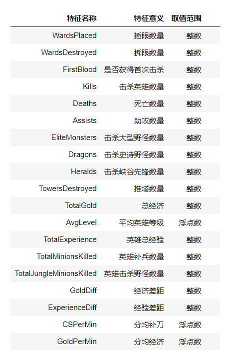
数据集变量描述如下:

; 数据集导入
mport numpy as np
import pandas as pd

import matplotlib.pyplot as plt
import seaborn as sns
df = pd.read_csv('./high_diamond_ranked_10min.csv')
y = df.blueWins
drop_cols = ['gameId','blueWins']
x = df.drop(drop_cols, axis=1)
x.describe()
- 不同对局中插眼数和拆眼数的取值范围存在明显差距,甚至有前十分钟插了250个眼的异常值。
- EliteMonsters的取值相当于Deagons + Heralds。
- TotalGold 等变量在大部分对局中差距不大。
- 两支队伍的经济差和经验差是相反数。
- 红队和蓝队拿到首次击杀的概率大概都是50%
可视化描述
data = x
data_std = (data - data.mean()) / data.std()
data = pd.concat([y, data_std.iloc[:, 0:9]], axis=1)
data = pd.melt(data, id_vars='blueWins', var_name='Features', value_name='Values')

fig, ax = plt.subplots(1,2,figsize=(15,5))

sns.violinplot(x='Features', y='Values', hue='blueWins', data=data, split=True,
               inner='quart', ax=ax[0], palette='Blues')
fig.autofmt_xdate(rotation=45)

data = x
data_std = (data - data.mean()) / data.std()
data = pd.concat([y, data_std.iloc[:, 9:18]], axis=1)
data = pd.melt(data, id_vars='blueWins', var_name='Features', value_name='Values')

sns.violinplot(x='Features', y='Values', hue='blueWins',
               data=data, split=True, inner='quart', ax=ax[1], palette='Blues')
fig.autofmt_xdate(rotation=45)

plt.show()

从图中可以看出:
- 击杀英雄数量越多更容易赢,死亡数量越多越容易输(bluekills与bluedeaths左右的区别)。
- 助攻数量与击杀英雄数量形成的图形状类似,说明他们对游戏结果的影响差不多。
- 一血的取得情况与获胜有正相关,但是相关性不如击杀英雄数量明显。
- 经济差与经验差对于游戏胜负的影响较小。
击杀野怪数量对游戏胜负的影响并不大。
plt.figure(figsize=(18,14))
sns.heatmap(round(x.corr(),2), cmap='Blues', annot=True)
plt.show()

drop_cols = ['redAvgLevel','blueAvgLevel']
x.drop(drop_cols, axis=1, inplace=True)
sns.set(style='whitegrid', palette='muted')

x['wardsPlacedDiff'] = x['blueWardsPlaced'] - x['redWardsPlaced']
x['wardsDestroyedDiff'] = x['blueWardsDestroyed'] - x['redWardsDestroyed']

data = x[['blueWardsPlaced','blueWardsDestroyed','wardsPlacedDiff','wardsDestroyedDiff']].sample(1000)
data_std = (data - data.mean()) / data.std()
data = pd.concat([y, data_std], axis=1)
data = pd.melt(data, id_vars='blueWins', var_name='Features', value_name='Values')

plt.figure(figsize=(10,6))
sns.swarmplot(x='Features', y='Values', hue='blueWins', data=data)
plt.xticks(rotation=45)
plt.show()

从插眼数量的散点图发现不存在插眼数量与游戏胜负间的显著规律。猜测由于钻石分段以上在哪插眼在哪好排眼都是套路,所以数据中前十分钟插眼数拔眼数对游戏的影响不大。所以我们暂时先把这些特征去掉。
drop_cols = ['blueWardsPlaced','blueWardsDestroyed','wardsPlacedDiff',
            'wardsDestroyedDiff','redWardsPlaced','redWardsDestroyed']
x.drop(drop_cols, axis=1, inplace=True)
x['killsDiff'] = x['blueKills'] - x['blueDeaths']
x['assistsDiff'] = x['blueAssists'] - x['redAssists']

x[['blueKills','blueDeaths','blueAssists','killsDiff','assistsDiff','redAssists']].hist(figsize=(12,10), bins=20)
plt.show()

发现击杀、死亡与助攻数的数据分布差别不大。但是击杀减去死亡、助攻减去死亡的分布与原分布差别很大,因此我们新构造这么两个特征。
data = x[['blueKills','blueDeaths','blueAssists','killsDiff','assistsDiff','redAssists']].sample(1000)
data_std = (data - data.mean()) / data.std()
data = pd.concat([y, data_std], axis=1)
data = pd.melt(data, id_vars='blueWins', var_name='Features', value_name='Values')

plt.figure(figsize=(10,6))
sns.swarmplot(x='Features', y='Values', hue='blueWins', data=data)
plt.xticks(rotation=45)
plt.show()
上图可以发现击杀数与死亡数与助攻数,以及我们构造的特征对数据都有较好的分类能力。
data = pd.concat([y, x], axis=1).sample(500)

sns.pairplot(data, vars=['blueKills','blueDeaths','blueAssists','killsDiff','assistsDiff','redAssists'],
             hue='blueWins')

plt.show()
x['dragonsDiff'] = x['blueDragons'] - x['redDragons']
x['heraldsDiff'] = x['blueHeralds'] - x['redHeralds']
x['eliteDiff'] = x['blueEliteMonsters'] - x['redEliteMonsters']

data = pd.concat([y, x], axis=1)

eliteGroup = data.groupby(['eliteDiff'])['blueWins'].mean()
dragonGroup = data.groupby(['dragonsDiff'])['blueWins'].mean()
heraldGroup = data.groupby(['heraldsDiff'])['blueWins'].mean()

fig, ax = plt.subplots(1,3, figsize=(15,4))

eliteGroup.plot(kind='bar', ax=ax[0])
dragonGroup.plot(kind='bar', ax=ax[1])
heraldGroup.plot(kind='bar', ax=ax[2])

print(eliteGroup)
print(dragonGroup)
print(heraldGroup)

plt.show()
构造了两队之间是否拿到龙、是否拿到峡谷先锋、击杀大型野怪的数量差值,发现在游戏的前期拿到龙比拿到峡谷先锋更容易获得胜利。拿到大型野怪的数量和胜率也存在着强相关。
x['towerDiff'] = x['blueTowersDestroyed'] - x['redTowersDestroyed']

data = pd.concat([y, x], axis=1)

towerGroup = data.groupby(['towerDiff'])['blueWins']
print(towerGroup.count())
print(towerGroup.mean())

fig, ax = plt.subplots(1,2,figsize=(15,5))

towerGroup.mean().plot(kind='line', ax=ax[0])
ax[0].set_title('Proportion of Blue Wins')
ax[0].set_ylabel('Proportion')

towerGroup.count().plot(kind='line', ax=ax[1])
ax[1].set_title('Count of Towers Destroyed')
ax[1].set_ylabel('Count')
推塔是英雄联盟这个游戏的核心,因此推塔数量可能与游戏的胜负有很大关系。我们绘图发现,尽管前十分钟推掉第一座防御塔的概率很低,但是一旦某只队伍推掉第一座防御塔,获得游戏的胜率将大大增加。
利用 LightGBM 进行训练与预测
from sklearn.model_selection import train_test_split
data_target_part = y
data_features_part = x

x_train, x_test, y_train, y_test = train_test_split(data_features_part, data_target_part, test_size = 0.2, random_state = 2020)
from lightgbm.sklearn import LGBMClassifier

clf = LGBMClassifier()

clf.fit(x_train, y_train)
train_predict = clf.predict(x_train)
test_predict = clf.predict(x_test)
from sklearn import metrics

print('The accuracy of the Logistic Regression is:',metrics.accuracy_score(y_train,train_predict))
print('The accuracy of the Logistic Regression is:',metrics.accuracy_score(y_test,test_predict))

confusion_matrix_result = metrics.confusion_matrix(test_predict,y_test)
print('The confusion matrix result:\n',confusion_matrix_result)

plt.figure(figsize=(8, 6))
sns.heatmap(confusion_matrix_result, annot=True, cmap='Blues')
plt.xlabel('Predicted labels')
plt.ylabel('True labels')
plt.show()
利用 LightGBM 进行特征选择
sns.barplot(y=data_features_part.columns, x=clf.feature_importances_)
from sklearn.metrics import accuracy_score
from lightgbm import plot_importance

def estimate(model,data):

    ax1=plot_importance(model,importance_type="gain")
    ax1.set_title('gain')
    ax2=plot_importance(model, importance_type="split")
    ax2.set_title('split')
    plt.show()
def classes(data,label,test):
    model=LGBMClassifier()
    model.fit(data,label)
    ans=model.predict(test)
    estimate(model, data)
    return ans

ans=classes(x_train,y_train,x_test)
pre=accuracy_score(y_test, ans)
print('acc=',accuracy_score(y_test,ans))
通过调整参数获得更好的效果
from sklearn.model_selection import GridSearchCV

learning_rate = [0.1, 0.3, 0.6]
feature_fraction = [0.5, 0.8, 1]
num_leaves = [16, 32, 64]
max_depth = [-1,3,5,8]

parameters = { 'learning_rate': learning_rate,
              'feature_fraction':feature_fraction,
              'num_leaves': num_leaves,
              'max_depth': max_depth}
model = LGBMClassifier(n_estimators = 50)

clf = GridSearchCV(model, parameters, cv=3, scoring='accuracy',verbose=3, n_jobs=-1)
clf = clf.fit(x_train, y_train)
clf.best_params_
clf = LGBMClassifier(feature_fraction = 0.8,
                    learning_rate = 0.1,
                    max_depth= 3,
                    num_leaves = 16)

clf.fit(x_train, y_train)

train_predict = clf.predict(x_train)
test_predict = clf.predict(x_test)

print('The accuracy of the Logistic Regression is:',metrics.accuracy_score(y_train,train_predict))
print('The accuracy of the Logistic Regression is:',metrics.accuracy_score(y_test,test_predict))

confusion_matrix_result = metrics.confusion_matrix(test_predict,y_test)
print('The confusion matrix result:\n',confusion_matrix_result)

plt.figure(figsize=(8, 6))
sns.heatmap(confusion_matrix_result, annot=True, cmap='Blues')
plt.xlabel('Predicted labels')
plt.ylabel('True labels')
plt.show()
至此就完成了一个简单的LightGBM算法的实践应用,感兴趣的同学可以去前文的参考链接里获取相应的数据集自行探索。
Original: https://blog.csdn.net/weixin_46719623/article/details/113558566
Author: 小黄油块跑
Title: 机器学习(三):基于LightGBM的分类预测
原创文章受到原创版权保护。转载请注明出处:https://www.johngo689.com/661588/
转载文章受原作者版权保护。转载请注明原作者出处!