

文章目录
*
– 一.数据集选择
–
+ 1.感知机
+ 2.K近邻(knn)
+ 3.朴素贝叶斯
+ 4.决策树id3
+ 5.逻辑斯蒂回归
+ 总结
一.数据集选择
鸢尾花数据集-iris.data
Iris数据集是常用的分类实验数据集,由Fisher, 1936收集整理。Iris也称鸢尾花卉数据集,是一类多重变量分析的数据集。数据集包含150个数据样本,分为3类,每类50个数据,每个数据包含4个属性(分别是:花萼长度,花萼宽度,花瓣长度,花瓣宽度)。可通过这4个属性预测鸢尾花卉属于(Setosa,Versicolour,Virginica)三个种类的鸢尾花中的哪一类。
Iris里有两个属性iris.data,iris.target。data是一个矩阵,每一列代表了萼片或花瓣的长宽,一共4列,每一列代表某个被测量的鸢尾植物,一共有150条记录。
数据集链接
数据集预处理:
由于数据集较小,易于划分,对测试集加入噪声后测试精确率
1.感知机
特点:
(1)二类分类线性模型。
(2)输入为实例的特征向量,输出为实例的类别。
(3)导入基于误分类的损失函数。
(4)利用梯度下降法对损失函数进行极小化。
算法实现:
import numpy as np
import matplotlib.pyplot as plt
import pandas as pd
from sklearn import metrics
df = pd.read_csv('../data/iris.data', header=None)
df.tail()
y = df.iloc[0:25, 4].values
y1 = df.iloc[75:100, 4].values
y = np.concatenate([y, y1])
y = np.where(y == 'Iris-setosa', -1, 1)
X = df.iloc[0:25, [0, 2]].values
X1 = df.iloc[75:100, [0, 2]].values
X = np.row_stack((X, X1))
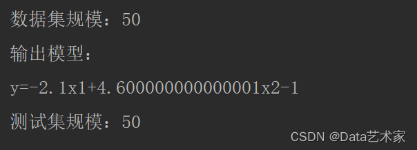
print("数据集规模:" + str(X.shape[0]))
p_x = np.array(X)
y = np.array(y)
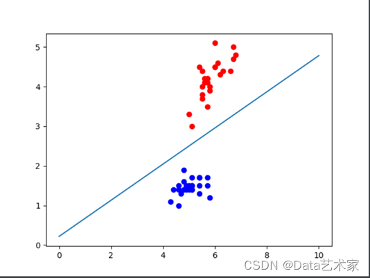
plt.figure()
for i in range(len(p_x)):
if y[i] == 1:
plt.plot(p_x[i][0], p_x[i][1], 'ro')
else:
plt.plot(p_x[i][0], p_x[i][1], 'bo')
w = np.array([0, 0])
b = 0
delta = 1
count = 0
while 1:
choice = -1
for j in range(len(p_x)):
if y[j] != np.sign(np.dot(w, p_x[j]) + b):
choice = j
w = w + delta * y[choice] * p_x[choice]
b = b + delta * y[choice]
break
if choice == -1:
break
for i in range(len(p_x)):
if y[i] == np.sign(np.dot(w, p_x[i]) + b):
count += 1
else:
count = 0
break
if count == len(p_x):
break
print("输出模型:")
print("y=" + str(round(w[0], 1)) + "x1+" + str(w[1]) + "x2" + str(b))
line_x = [0, 10]
line_y = [0, 0]
for i in range(len(line_x)):
line_y[i] = (-w[0] * line_x[i] - b) / w[1]
plt.plot(line_x, line_y)
plt.savefig("picture.png")
y = df.iloc[25:50, 4].values
y1 = df.iloc[50:75, 4].values
y = np.concatenate([y, y1])
y = np.where(y == 'Iris-setosa', -1, 1)
X = df.iloc[25:50, [0, 2]].values
X1 = df.iloc[50:75, [0, 2]].values
X = np.row_stack((X, X1))
print("测试集规模:" + str(X.shape[0]))
print()
p_x = np.array(X)
y = np.array(y)
zhen = 0
fu = 0
y_predict = []
for i in range(len(p_x)):
print("测试数据:" + str([p_x[i][0], p_x[i][1]]))
print("真实结果:" + str(y[i]))
y_predict.append(int(np.sign(np.dot(w, p_x[i]) + b)))
print("预测结果:" + str(y_predict[i]))
print()
M = metrics.confusion_matrix(y_predict, y)
print('混淆矩阵:\n', M)
n = len(M)
for i in range(n):
rowsum, colsum = sum(M[i]), sum(M[r][i] for r in range(n))
precision = M[i][i] / float(colsum)
recall = M[i][i] / float(rowsum)
F1 = precision * recall * 2 / (precision + recall)
print('y=%d 精确率: %s' % (i, precision), '召回率: %s' % recall, 'F1值: %s' % F1)
print("感知机模型精度:{:.5f}".format(np.mean(y_predict == y)))
分类图像展示:

运行结果:
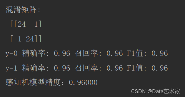
类别 精确率 召回率 F1 0 0.96 0.96 0.96 1 0.96 0.96 0.96
模型精度(准确率):0.96000
2.K近邻(knn)
特点:
优点:
(1)简单好用,容易理解,精度高,理论成熟,既可以用来做分类也可以用来做回归;
(2)可用于数值型数据和离散型数据;
(3)训练时间复杂度为O(n);无数据输入假定;
(4)对异常值不敏感。
缺点:
(1)计算复杂性高;空间复杂性高;
(2)样本不平衡问题(即有些类别的样本数量很多,而其它样本的数量很少);
(3)一般数值很大的时候不用这个,计算量太大。但是单个样本又不能太少,否则容易 发生误分。
(4)最大的缺点是无法给出数据的内在含义。
算法实现:
import pandas as pd
import numpy as np
import operator
import json
from numpy import *

def createDataSet():

    df = pd.read_csv('../data/iris.data',
                     header=None)
    df.tail()

    y = df.iloc[0:25, 4].values
    y1 = df.iloc[75:100, 4].values
    y = np.concatenate([y, y1])

    y = np.where(y == 'Iris-setosa', -1, 1)
    X = df.iloc[0:25, [0, 2]].values
    X1 = df.iloc[75:100, [0, 2]].values
    X = np.row_stack((X, X1))

    data = np.array(X)
    labels = np.array(y)
    labels1 = []
    for i in labels:
        if labels[i] == 1:
            labels1.append(1)
        else:
            labels1.append(-1)

    return data, labels1

def classify(inX, data, labels, k):
    dataSetSize = data.shape[0]

    diffmat = tile(inX, (dataSetSize, 1)) - data

    sqDiffMat = diffmat ** 2

    sqDistances = sqDiffMat.sum(axis=1)

    distances = sqDistances ** 0.5

    sortedDistIndexes = distances.argsort()

    classCount = {}
    for i in range(k):

        voteLabel = labels[sortedDistIndexes[i]]
        classCount[voteLabel] = classCount.get(voteLabel, 0) + 1
    print('标签出现的次数:')
    print(json.dumps(classCount, ensure_ascii=False))
    sortedClassCount = sorted(classCount.items(), key=operator.itemgetter(1), reverse=True)

    print('排序后:')
    print(json.dumps(sortedClassCount, ensure_ascii=False))

    return sortedClassCount[0][0]
测试
import pandas as pd
from sklearn import metrics

import knn
import numpy as np

data, labels = knn.createDataSet()

df = pd.read_csv('../data/iris.data', header=None)
df.tail()

y = df.iloc[25:50, 4].values
y1 = df.iloc[50:75, 4].values
y = np.concatenate([y, y1])

y = np.where(y == 'Iris-setosa', 1, -1)

X = df.iloc[25:50, [0, 2]].values
X1 = df.iloc[50:75, [0, 2]].values
X = np.row_stack((X, X1))

p_x = np.array(X)
y = np.array(y)
train_data, train_lable = knn.createDataSet()

y_predict = []
for i in range(len(p_x)):
    print("测试数据:"+str([p_x[i][0], p_x[i][1]]))
    print("真实结果:" + str(y[i]))
    y_predict.append(knn.classify([p_x[i][0], p_x[i][1]], train_data, train_lable, 3))
    print('预测结果:' + str(y_predict[i])+"\n")

M = metrics.confusion_matrix(y_predict, y)
print('混淆矩阵:\n', M)

n = len(M)
for i in range(n):
    rowsum, colsum = sum(M[i]), sum(M[r][i] for r in range(n))
    precision = M[i][i] / float(colsum)
    recall = M[i][i] / float(rowsum)
    F1 = precision * recall * 2 / (precision + recall)
    print('y=%d 精确率: %s' % (i, precision), '召回率: %s' % recall, 'F1值: %s' % F1)
print("KNN模型精度:{:.5f}".format(np.mean(y_predict == y)))
运行结果
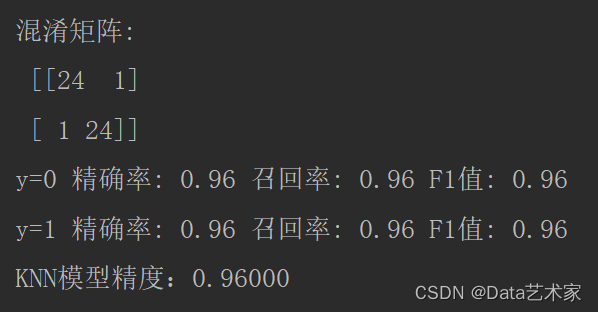
类别 精确率 召回率 F1 0 0.96 0.96 0.96 1 0.96 0.96 0.96
模型精度(准确率):0.96000
3.朴素贝叶斯
特点:
朴素贝叶斯的主要优势有:
1)朴素贝叶斯模型有稳定的分类效率。
2)对小规模的数据表现很好,能处理多分类任务,适合增量式训练,尤为是数据量超出内存时,能够一批批的去增量训练。
3)对缺失数据不太敏感,算法也比较简单,经常使用于文本分类。
朴素贝叶斯的主要缺点有:
1) 理论上,朴素贝叶斯模型与其余分类方法相比具备最小的偏差率。可是实际上并不是老是如此,这是由于朴素贝叶斯模型给定输出类别的状况下,假设属性之间相互独立,这个假设在实际应用中每每是不成立的,在属性个数比较多或者属性之间相关性较大时,分类效果很差。而在属性相关性较小时,朴素贝叶斯性能最为良好。对于这一点,有半朴素贝叶斯之类的算法经过考虑部分关联性适度改进。
2)须要知道先验几率,且先验几率不少时候取决于假设,假设的模型能够有不少种,所以在某些时候会因为假设的先验模型的缘由致使预测效果不佳。
3)因为咱们是经过先验和数据来决定后验的几率从而决定分类,因此分类决策存在必定的错误率。
4)对输入数据的表达形式很敏感。
代码展示:
import numpy as np
import pandas as pd
from sklearn import metrics

def createDataSet():

    df = pd.read_csv('../data/iris.data',
                     header=None)
    df.tail()

    y = df.iloc[0:25, 4].values
    y1 = df.iloc[75:100, 4].values
    y = np.concatenate([y, y1])
    y = np.where(y == 'Iris-setosa', -1, 1)
    X = df.iloc[0:25, [0, 2]].values
    X1 = df.iloc[75:100, [0, 2]].values
    X = np.row_stack((X, X1))
    dataSet = np.column_stack((X, y))
    labels = ['x1', 'x2', 'y']
    return dataSet, labels

def typeCount(typeList, t):
    cnt = 0
    for tL in typeList:
        if tL == t:
            cnt += 1
    return cnt

def featCount(dataSet, i, feat, y):
    cnt = 0

    for row in dataSet:
        if row[i] == feat and row[-1] == y:
            cnt += 1
    return cnt

def calcBayes(dataSet, X):

    lenDataSet = len(dataSet)
    typeList = [row[-1] for row in dataSet]
    typeSet = set(typeList)
    print(typeList, typeSet)
    typeLen = len(typeSet)

    pList = []
    for t in typeSet:
        yNum = typeCount(typeList, t)
        print(f'{t} num =', yNum)
        py = yNum / lenDataSet
        print(f'P(Y = {t}) =', py)
        pSum = py

        for i in range(len(X)):
            xiNum = featCount(dataSet, i, X[i], t)
            print(f'特征{X[i]} num =', xiNum)

            pxy = xiNum / yNum
            print(f'条件概率 =', pxy)
            pSum *= pxy
        pList.append(pSum)

    return pList, typeSet

def predict(pList, typeList):
    for i in range(len(pList)):
        if pList[i] == max(pList):
            print(f'预测类 为 = {typeList[i]}')
            print('*' * 50)
            return typeList[i]

if __name__ == '__main__':

    df = pd.read_csv('../data/iris.data',
                     header=None)
    df.tail()

    y = df.iloc[25:50, 4].values
    y1 = df.iloc[50:75, 4].values
    y = np.concatenate([y, y1])

    y = np.where(y == 'Iris-setosa', -1, 1)

    X = df.iloc[25:50, [0, 2]].values
    X1 = df.iloc[50:75, [0, 2]].values
    X = np.row_stack((X, X1))

    p_x = np.array(X)
    y = np.array(y)
    data = np.column_stack((p_x, y))
    data = np.array(data)
    dataSet, labels = createDataSet()
    predict_result = []

    for i in data:
        pList, typeSet = calcBayes(dataSet, [i[0], i[1]])
        predict_result.append(predict(pList, list(typeSet)))

    M = metrics.confusion_matrix(predict_result, y)
    print('混淆矩阵:\n', M)

    n = len(M)
    for i in range(n):
        rowsum, colsum = sum(M[i]), sum(M[r][i] for r in range(n))
        precision = M[i][i] / float(colsum)
        recall = M[i][i] / float(rowsum)
        F1 = precision * recall * 2 / (precision + recall)
        print('y=%d 精确率: %s' % (i, precision), '召回率: %s' % recall, 'F1值: %s' % F1)
    print("朴素贝叶斯模型精度:{:.5f}".format(np.mean(predict_result == y)))
运行结果:
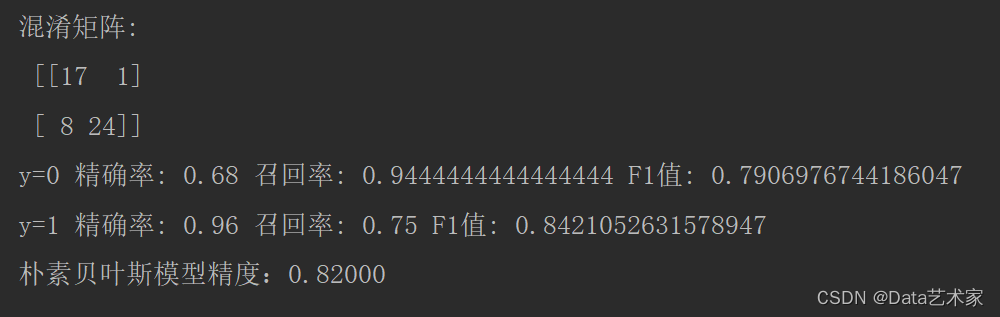
类别 精确率 召回率 F1 0 0.68 0.94 0.79 1 0.96 0.75 0.84
模型精度(准确率):0.82000
4.决策树id3
特点:
决策树的核心思想是:相似的输入必然产生相似的输出。决策树通过把数据样本分配到树状结构的某个叶子节点来确定数据集中样本所属的分类。决策树可用于回归和分类。当用于回归时,预测结果为叶子节点所有样本的均值。
①优点
• 简单易懂,容易解释,可视化,适用性广。
• 可用于分类、回归问题。
②缺点
• 容易过拟合。
• 数据中的小变化会影响结果,不稳定。
• 每一个节点的选择都是贪婪算法,不能保证全局最优解。
使用场景:
适合于标称型(在有限目标集中取值)属性较多的样本数据。
具有较广的适用性,当对模型不确定时可以使用决策树进行验证。
代码实现
import math
from math import log
import operator

import numpy as np
import pandas as pd
from sklearn import metrics

import 决策树可视化 as treePlot

"""
函数说明:创建测试数据集
"""

def createDataSet():

    df = pd.read_csv('../data/iris.data',
                     header=None)
    df.tail()

    y = df.iloc[0:25, 4].values
    y1 = df.iloc[75:100, 4].values
    y = np.concatenate([y, y1])
    y = np.where(y == 'Iris-setosa', 1, -1)
    X = df.iloc[0:25, 0:4].values
    X1 = df.iloc[75:100, 0:4].values
    X = np.row_stack((X, X1))
    print(X.shape[0])
    for i in range(X.shape[0]):
        for j in range(X.shape[1]):
            X[i][j] = math.ceil(X[i][j])
    dataSet = np.column_stack([X, y])
    dataSet = np.array(dataSet).tolist()

    labels = ['A1', 'A2', 'A3', 'A4']
    return dataSet, labels

"""
函数说明:计算给定数据集的经验熵(香农熵)
Parameters:
    dataSet - 数据集
Returns:
    shannonEnt - 经验熵(香农熵)
"""

def calcShannonEnt(dataSet):
    numEntires = len(dataSet)
    labelCounts = {}
    for featVec in dataSet:
        currentLabel = featVec[-1]
        if currentLabel not in labelCounts.keys():
            labelCounts[currentLabel] = 0
        labelCounts[currentLabel] += 1
    shannonEnt = 0.0
    for key in labelCounts:
        prob = float(labelCounts[key]) / numEntires
        shannonEnt -= prob * log(prob, 2)
    return shannonEnt

"""
函数说明:按照给定特征划分数据集
Parameters:
    dataSet - 待划分的数据集
    axis - 划分数据集的特征
    value - 需要返回的特征的值
"""

def splitDataSet(dataSet, axis, value):
    retDataSet = []
    for featVec in dataSet:
        if featVec[axis] == value:
            reducedFeatVec = featVec[:axis]
            reducedFeatVec.extend(featVec[axis + 1:])
            retDataSet.append(reducedFeatVec)
    return retDataSet

"""
函数说明:选择最优特征
Parameters:
    dataSet - 数据集
Returns:
    bestFeature - 信息增益最大的(最优)特征的索引值
"""

def chooseBestFeatureToSplit(dataSet):
    numFeatures = len(dataSet[0]) - 1
    baseEntropy = calcShannonEnt(dataSet)
    bestInfoGain = 0.0
    bestFeature = -1
    for i in range(numFeatures):

        featList = [example[i] for example in dataSet]
        uniqueVals = set(featList)
        newEntropy = 0.0
        for value in uniqueVals:
            subDataSet = splitDataSet(dataSet, i, value)
            prob = len(subDataSet) / float(len(dataSet))
            newEntropy += prob * calcShannonEnt(subDataSet)
        infoGain = baseEntropy - newEntropy
        print("第%d个特征的增益为%.3f" % (i, infoGain))
        if (infoGain > bestInfoGain):
            bestInfoGain = infoGain
            bestFeature = i
    return bestFeature

"""
函数说明:统计classList中出现此处最多的元素(类标签)
Parameters:
    classList - 类标签列表
Returns:
    sortedClassCount[0][0] - 出现此处最多的元素(类标签)
"""

def majorityCnt(classList):
    classCount = {}
    for vote in classList:
        if vote not in classCount.keys():
            classCount[vote] = 0
        classCount[vote] += 1
    sortedClassCount = sorted(classCount.items(), key=operator.itemgetter(1), reverse=True)
    return sortedClassCount[0][0]

"""
函数说明:递归构建决策树
Parameters:
    dataSet - 训练数据集
    labels - 分类属性标签
    featLabels - 存储选择的最优特征标签
Returns:
    myTree - 决策树
"""

def createTree(dataSet, labels, featLabels):
    classList = [example[-1] for example in dataSet]
    if classList.count(classList[0]) == len(classList):
        return classList[0]
    if len(dataSet[0]) == 1:
        return majorityCnt(classList)
    bestFeat = chooseBestFeatureToSplit(dataSet)
    bestFeatLabel = labels[bestFeat]
    featLabels.append(bestFeatLabel)
    myTree = {bestFeatLabel: {}}
    del (labels[bestFeat])
    featValues = [example[bestFeat] for example in dataSet]
    uniqueVals = set(featValues)
    for value in uniqueVals:
        subLabels = labels[:]

        myTree[bestFeatLabel][value] = createTree(splitDataSet(dataSet, bestFeat, value), subLabels, featLabels)
    return myTree

"""
函数说明:使用决策树执行分类
Parameters:
    inputTree - 已经生成的决策树
    featLabels - 存储选择的最优特征标签
    testVec - 测试数据列表,顺序对应最优特征标签
Returns:
    classLabel - 分类结果
"""

def classify(inputTree, featLabels, testVec):
    global classLabel
    firstStr = next(iter(inputTree))
    secondDict = inputTree[firstStr]
    featIndex = featLabels.index(firstStr)
    for key in secondDict.keys():
        if testVec[featIndex] == key:
            if type(secondDict[key]).__name__ == 'dict':
                classLabel = classify(secondDict[key], featLabels, testVec)
            else:
                classLabel = secondDict[key]
    return classLabel

if __name__ == '__main__':
    dataSet, labels = createDataSet()
    featLabels = []
    myTree = createTree(dataSet, labels, featLabels)
    treePlot.createPlot(myTree)
    print(myTree)

    df = pd.read_csv('../data/iris.data',
                     header=None)
    df.tail()

    y = df.iloc[25:50, 4].values
    y1 = df.iloc[50:75, 4].values
    y = np.concatenate((y, y1))
    y = np.where(y == 'Iris-setosa', 1, -1)
    X = df.iloc[25:50, 2].values
    X1 = df.iloc[50:75, 2].values
    X = np.concatenate([X, X1])
    for i in range(X.shape[0]):
        X[i] = math.ceil(X[i])

    predict_result = []
    for i in X:
        i = [i]
        result = classify(myTree, featLabels, i)
        print(result)
        if result == 1.0:
            predict_result.append(1.0)
        else:
            predict_result.append(-1.0)
    M = metrics.confusion_matrix(predict_result, y)
    print('混淆矩阵:\n', M)

    n = len(M)
    for i in range(n):
        rowsum, colsum = sum(M[i]), sum(M[r][i] for r in range(n))
        precision = M[i][i] / float(colsum)
        recall = M[i][i] / float(rowsum)
        F1 = precision * recall * 2 / (precision + recall)
        print('y=%d 精确率: %s' % (i, precision), '召回率: %s' % recall, 'F1值: %s' % F1)
    print("决策树Id3模型精度:{:.5f}".format(np.mean(predict_result == y)))
决策树可视化
import matplotlib.pyplot as plt
from matplotlib.font_manager import FontProperties
from matplotlib.font_manager import FontProperties
import matplotlib.pyplot as plt

decisionNode = dict(boxstyle='sawtooth', fc='0.8')
leafNode = dict(boxstyle='round4', fc='0.8')
arrow_args = dict(arrowstyle=')

font = FontProperties(fname=r"c:\windows\fonts\simsun.ttc", size=14)

"""
函数说明:获取决策树叶子结点的数目
Parameters:
    myTree - 决策树
Returns:
    numLeafs - 决策树的叶子结点的数目
"""

def getNumLeafs(myTree):
    numLeafs = 0

    firstStr = next(iter(myTree))
    secondDict = myTree[firstStr]
    for key in secondDict.keys():
        if type(secondDict[key]).__name__ == 'dict':
            numLeafs += getNumLeafs(secondDict[key])
        else:
            numLeafs += 1
    return numLeafs

"""
函数说明:获取决策树的层数
Parameters:
    myTree - 决策树
Returns:
    maxDepth - 决策树的层数
"""

def getTreeDepth(myTree):
    maxDepth = 0

    firstStr = next(iter(myTree))
    secondDict = myTree[firstStr]
    for key in secondDict.keys():
        if type(secondDict[key]).__name__ == 'dict':
            thisDepth = 1 + getTreeDepth(secondDict[key])
        else:
            thisDepth = 1
        if thisDepth > maxDepth:
            maxDepth = thisDepth
    return maxDepth

"""
函数说明:绘制结点
Parameters:
    nodeTxt - 结点名
    centerPt - 文本位置
    parentPt - 标注的箭头位置
    nodeType - 结点格式
"""

def plotNode(nodeTxt, centerPt, parentPt, nodeType):
    arrow_args = dict(arrowstyle=")
    font = FontProperties(fname=r"c:\windows\fonts\simsun.ttc", size=14)
    createPlot.ax1.annotate(nodeTxt, xy=parentPt, xycoords='axes fraction',
                            xytext=centerPt, textcoords='axes fraction',
                            va="center", ha="center", bbox=nodeType, arrowprops=arrow_args, fontproperties=font)

"""
函数说明:标注有向边属性值
Parameters:
    cntrPt、parentPt - 用于计算标注位置
    txtString - 标注的内容
"""

def plotMidText(cntrPt, parentPt, txtString):
    xMid = (parentPt[0] - cntrPt[0]) / 2.0 + cntrPt[0]
    yMid = (parentPt[1] - cntrPt[1]) / 2.0 + cntrPt[1]
    createPlot.ax1.text(xMid, yMid, txtString, va="center", ha="center", rotation=30)

"""
函数说明:绘制决策树
Parameters:
    myTree - 决策树(字典)
    parentPt - 标注的内容
    nodeTxt - 结点名
"""

def plotTree(myTree, parentPt, nodeTxt):
    decisionNode = dict(boxstyle="sawtooth", fc="0.8")
    leafNode = dict(boxstyle="round4", fc="0.8")
    numLeafs = getNumLeafs(myTree)
    depth = getTreeDepth(myTree)
    firstStr = next(iter(myTree))
    cntrPt = (plotTree.xOff + (1.0 + float(numLeafs)) / 2.0 / plotTree.totalW, plotTree.yOff)
    plotMidText(cntrPt, parentPt, nodeTxt)
    plotNode(firstStr, cntrPt, parentPt, decisionNode)
    secondDict = myTree[firstStr]
    plotTree.yOff = plotTree.yOff - 1.0 / plotTree.totalD
    for key in secondDict.keys():
        if type(secondDict[key]).__name__ == 'dict':
            plotTree(secondDict[key], cntrPt, str(key))
        else:
            plotTree.xOff = plotTree.xOff + 1.0 / plotTree.totalW
            plotNode(secondDict[key], (plotTree.xOff, plotTree.yOff), cntrPt, leafNode)
            plotMidText((plotTree.xOff, plotTree.yOff), cntrPt, str(key))
    plotTree.yOff = plotTree.yOff + 1.0 / plotTree.totalD

"""
函数说明:创建绘制面板
Parameters:
    inTree - 决策树(字典)
"""

def createPlot(inTree):
    fig = plt.figure(1, facecolor='white')
    fig.clf()
    axprops = dict(xticks=[], yticks=[])
    createPlot.ax1 = plt.subplot(111, frameon=False, **axprops)
    plotTree.totalW = float(getNumLeafs(inTree))
    plotTree.totalD = float(getTreeDepth(inTree))
    plotTree.xOff = -0.5 / plotTree.totalW;
    plotTree.yOff = 1.0;
    plotTree(inTree, (0.5, 1.0), '')
    plt.show()
生成决策树:
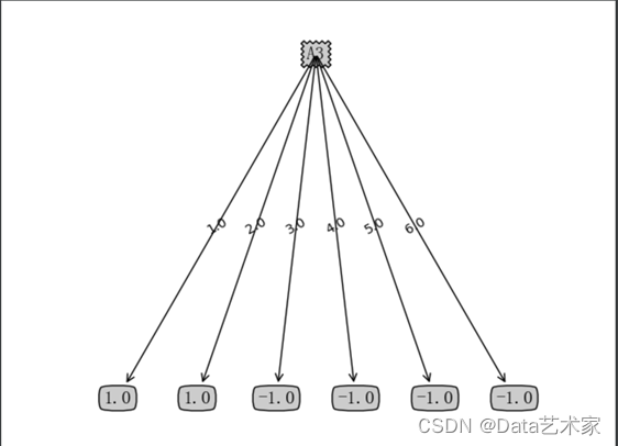
因为数据集仅对A3特征存在可分,所以此数据集对于决策树只生成一个节点
运行结果:
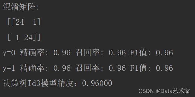
类别 精确率 召回率 F1 0 0.96 0.96 0.96 1 0.96 0.96 0.96
模型精度(准确率):0.96000
5.逻辑斯蒂回归
特点:
逻辑斯谛回归是经典的分类方法,它属于对数线性模型,原理是根据现有的数据对分类边界线建立回归公式,以此进行分类。(主要思想)
定义:
在线性回归模型的基础上,使用Sigmoid函数,将线性模型的结果压缩到[0,1]之间,使其拥有概率意义,它可以将任意输入映射到[0,1]区间,实现值到概率转换。
- 属于概率性判别式模型
- 线性分类算法
在学习逻辑回归模型之前,先来看一下逻辑斯谛分布,因为我们的逻辑斯蒂模型就是根据逻辑斯蒂分布得到的;通过参数估计方法直接估计出参数,从而得到P(Y|X)。
import pandas as pd
from sklearn import metrics
from sklearn.linear_model import LogisticRegression
from math import exp
from math import *
from sklearn.datasets import load_iris
from sklearn.model_selection import train_test_split
from numpy import *
import numpy as np

class LogisticRegressionClassifier(object):
    def __init__(self, eta=0.1, loop=30):
        self.eta = eta
        self.loop = loop

    def sigmoid(self, x):
        return 1.0 / (1 + exp(-x))

    def data_tranforce(self, x_train):
        data = []
        d = []
        for x in x_train:
            data.append([1.0, *x])

        return data

    def fit(self, x_train, y_train):
        data_mat = self.data_tranforce(x_train)
        n = shape(data_mat)[1]
        self.weight = ones((n, 1))
        cls = self.loop
        for k in range(cls):
            for i in range(len(x_train)):
                h = self.sigmoid(np.dot(data_mat[i], self.weight))
                err = (y_train[i] - h)

                self.weight += self.eta * err * np.transpose([data_mat[i]])

    def test(self, x_test, y_test):
        numbers = 0
        x_test = self.data_tranforce(x_test)
        y_predict = []
        for x, y in zip(x_test, y_test):
            result = np.dot(x, self.weight)
            if result > 0 and y == 1 or result > 0 and y == 0:
                y_predict.append(1)
            if result < 0 and y == 0 or result < 0 and y == 1:
                y_predict.append(0)
        return np.array(y_predict)

def main():
    df = pd.read_csv('../data/iris.data',
                     header=None)
    df.tail()
    x = df.iloc[:100, :2].values
    y = df.iloc[:100, 4].values
    y = np.where(y == 'Iris-setosa', 1, 0)
    x_train = x[0:25]
    x_train = np.concatenate((x_train, x[75:100]))
    x_test = x[25:75]
    y_train = y[0:25]
    y_train = np.concatenate((y_train, y[75:100]))
    y_test = np.array(y[25:75])
    print('train', y_train)
    print('test', y_test)
    my_l = LogisticRegressionClassifier()
    my_l.fit(x_train, y_train)

    y_predict = my_l.test(x_test, y_test)
    print('ptedict', y_predict)
    M = metrics.confusion_matrix(y_predict, y_test)
    print('混淆矩阵:\n', M)

    n = len(M)
    for i in range(n):
        rowsum, colsum = sum(M[i]), sum(M[r][i] for r in range(n))
        precision = M[i][i] / float(colsum)
        recall = M[i][i] / float(rowsum)
        F1 = precision * recall * 2 / (precision + recall)
        print('y=%d 精确率: %s' % (i, precision), '召回率: %s' % recall, 'F1值: %s' % F1)
    print("逻辑斯蒂回归模型精度:{:.5f}".format(np.mean(y_predict == y_test)))

if __name__ == "__main__":
    main()
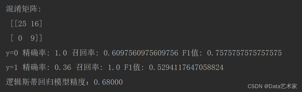
类别 精确率 召回率 F1 0 1 0.61 0.76 1 0.36 1 0.52
模型精度(准确率):0.68000
总结
机器学习算法有很多,本学期及本实验以分类算法为主,讲解了经典的分类算法,如感知机,knn,朴素贝叶斯,决策树,逻辑斯蒂回归,最大熵模型,SVM(支持向量机),AdaBoost ,k-means(聚类算法)等,通过对于分类算法的学习,我学习到了各算法的原理以及实现,还有与其他算法的比较,及一些相关知识点:
随机梯度下降(SGD):
是一种简单但又非常高效的方法,主要用于凸损失函数下线性分类器的判别式学习,例如(线性) 支持向量机和逻辑斯蒂回归。
优势:
• 高效。
• 易于实现 (有大量优化代码的机会)。
劣势:
• SGD 需要一些超参数,例如正则化参数和迭代次数。
• SGD 对特征缩放敏感。
最小二乘法与梯度下降法比较:
最小二乘法跟梯度下降法都是通过求导来求损失函数的最小值, 首先它们都是机器学习中,计算问题最优解的优化方法,但它们采用的方式不同,前者采用暴力的解方程组方式,直接,简单,粗暴,在条件允许下,求得最优解;而后者采用步进迭代的方式,一步一步的逼近最优解。实际应用中,大多问题是不能直接解方程求得最优解的,所以梯度下降法应用广泛。
KNN最近邻:
原理是从训练样本中找到与新点在距离上最近的预定数量的几个点,然后从这些点中预测标签。 这些点的数量可以是用户自定义的常量(K-最近邻学习), 也可以根据不同的点的局部密度(基于半径的最近邻学习)确定。距离通常可以通过任何度量来衡量: 标准欧式距离是最常见的选择。尽管它简单,但最近邻算法已经成功地适用于很多的分类和回归问题,例如手写数字或卫星图像的场景。 作为一个非参数化方法,它经常成功地应用于决策边界非常不规则的分类情景下。最近邻分类属于 基于实例的学习 或 非泛化学习 :它不会去构造一个泛化的内部模型,而是简单地存储训练数据的实例。 分类是由每个点的最近邻的简单多数投票中计算得到的:一个查询点的数据类型是由它最近邻点中最具代表性的数据类型来决定的。
朴素贝叶斯:
朴素贝叶斯方法是基于贝叶斯定理的一组有监督学习算法,即”简单”地假设每对特征之间相互独立。基于训练集所求得概率,根据贝叶斯概率模型求得测试集各类别概率大小,取概率最大的类别为预测类别;朴素贝叶斯算法假设了数据集属性之间是相互独⽴的,因此算法的逻辑性⼗分简单,并且算法较为稳定,当数据呈现不同的特点时,朴素贝叶斯的分类性能不会有太⼤的差异。换句话说就是朴素贝叶斯算法的健壮性⽐较好,对于不同类型的数据集不会呈现出太⼤的差异性。当数据集属性之间的关系相对⽐较独⽴时,朴素贝叶斯分类算法会有较好的效果。
缺点:性独⽴性的条件同时也是朴素贝叶斯分类器的不⾜之处。数据集属性的独⽴性在很多情况下是很难满⾜的,因为数据集的属性之间往往都存在着相互关联,如果在分类过程中出现这种问题,会导致分类的效果⼤⼤降低。
决策树:
信息熵(info entropy)
首先介绍一下信息熵的概念. 我们把样本抽取过程当做一次随机试验A, 那么A有k个可能的输出A1,A2,…,Ak . 对应于k个分类. 那么A的信息熵定义为:
信息增益:决策树根据各特征的信息增益大小选择决策树节点
基尼指数:不管是信息熵还是基尼指数, 他们都是不纯函数的一种表达, 不纯度变化的计算没有任何变化. 我们也可以自己撰写不纯度函数.
一般来说, 机器学习都需要特征归一化, 目的是让特征之间的比较可以在同一个量纲上进行. 但是从数据构建过程来看, 不纯函数的计算和比较都是单特征的. 所有决策树不需要数据的归一化.
决策树的主要问题是容易形成过拟合. 如果我们通过各种剪枝和条件限制, 虽然可以避免过拟合, 但是会牺牲特征的有效性.
算法精确度比较:
算法感知机朴素贝叶斯Knn决策树逻辑斯蒂回归精确度0.960.820.960.960.68
根据结果可以看出朴素贝叶斯与逻辑斯蒂回归算法精度相对来说其他算法较低;其他算法由于数据集并不是很大,并且同一数据集有可能逻辑斯蒂回归是一种对数线性模型。
由此总结出逻辑斯蒂回归的缺点:
1)容易欠拟合,分类精度不高。
2)数据特征有缺失或者特征空间很大时表现效果并不好。
经典的逻辑斯蒂回归模型(LR)可以用来解决二分类问题,但是它输出的并不是确切类别,而是一个概率。 在分析LR原理之前,先分析一下线性回归。线性回归能将输入数据通过对各个维度的特征分配不同的权重来进行表征,使得所有特征协同作出最后的决策。但是,这种表征方式是对模型的一个拟合结果,不能直接用于分类。在LR中,将线性回归的结果通过sigmod函数映射到0到1之间,映射的结果刚好可以看做是数据样本点属于某一类的概率,如果结果越接近0或者1,说明分类结果的可信度越高。这样做不仅应用了线性回归的优势来完成分类任务,而且分类的结果是0~1之间的概率,可以据此对数据分类的结果进行打分。对于线性不可分的数据,可以对非线性函数进行线性加权,得到一个不是超平面的分割面。 因此对于逻辑斯蒂回归分类一些数据可能并不是很准确。
Original: https://blog.csdn.net/weixin_52762273/article/details/126125612
Author: Data艺术家
Title: 【机器学习】二分类算法实现及算法精度比较
原创文章受到原创版权保护。转载请注明出处:https://www.johngo689.com/661459/
转载文章受原作者版权保护。转载请注明原作者出处!