【语义分割】类别不平衡损失函数合集

在语义分割领域，我们会常常遇到类别不平衡的问题。比如要分割的目标（前景）可能只占图像的一小部分，因此负样本的比重很大，导致网络倾向于将所有样本判断为负样本。本文介绍了在数据不平衡时常用的一些损失函数。

类别不平衡会出现什么问题呢？假设我们需要训练一个分类器来对黄豆和绿豆分类，用100颗豆子训练分类器，其中99颗黄豆、1颗绿豆，那么分类器会倾向于把所有豆子都分类为黄豆，因为这么做就可以达到99%的准确率。但是我们不希望分类器这么做，所以需要一些方法来提升分类器的性能。

目录

一、Weighted Cross Entropy Loss

二、Focal Loss

三、Dice Loss

总结

参考：

四、Lovasz Loss

源码分析（多分类）

五、OHEM（Online Hard Example Mining）

六、Semantic Encoding Loss

七、Pixel Contrast Cross Entropy Loss

网络结构

对比损失

采样策略

声明

一、Weighted Cross Entropy Loss

交叉熵损失函数的实现可以参考【深度学习损失函数numpy实现并与torch对比】，当语义分割数据不平衡时，可以计算各个类别在数据集中所占的比例，然后将比率取倒数作为权重。

二、Focal Loss

语义分割多分类Focal Losss代码：PaddleSeg Focal Loss

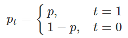
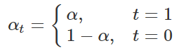
何凯明大神的RetinaNet中提出了Focal Loss来解决类别不平衡的问题，下式为focal loss的公式，α为类别的权重，γ为大于0的值，在2分类的情况下：

首先给出

公式如下，则：

再给出

公式如下，则：

论文给出的focal loss公式：

将

和带入上式，有：

将t=0和t=1分别带入，得到下式（y=p，

）(下式来源)：

对于多分类的情况，可根据BinaryCrossEntropy推广到多分类交叉熵的方法推广。

focal loss是如何起作用的呢？

首先对其求导，为了计算方便，简化上式：去掉常数α，设置γ为2，用ln代替log，得到下式：

对其求导：

可以看出，

接近1时，focal loss的梯度趋于0，靠近0，focal loss的梯度越来越大。那么预测和真实值非常接近的时候，梯度极小，网络参数几乎不变，当预测值和真实值差距较大时，梯度变大，网络参数开始调整。

三、Dice Loss

dice loss 来自文章V-Net: Fully Convolutional Neural Networks for Volumetric Medical Image Segmentation，旨在应对语义分割中正负样本强烈不平衡的场景。

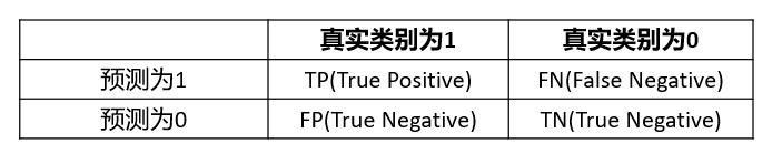
对于二分类问题，TP\FP\FN\TN定义如下：

对于语义分割任务，可看下图，蓝色和绿色为预测区域（FP+TP），橙色为真实类别区域，那么dice coefficient的定义为：

可以看出dice coefficient是可以体现出预测区域和真实区域的重叠程度，它的取值范围是[0, 1]，当dice coefficient为1时，说明预测区域和真实区域完全重叠，是理想状态；当dice coefficient为0时，说明预测结果一点作用没有。

dice coefficient在数据不平衡时能够给出均衡的评价。

给定优化指标本身与代理损失函数之间的选择，最优选择就是指标本身。既然dice coefficient越大越好，且数据不平衡不会影响到它，那么可以把dice作为优化目标。神经网络训练时的目标就是使损失函数最小，但是这里的dice coefficient是越大越好，所以对他进行一点小修改得到dice loss：

为了防止分子分母出现0，再在分子分母加上一个很小的数，得到：

上面的函数是离散的，不能作为神经网络的优化目标，把网络输出的概率值带进去，使它连续（p为网络输出的概率值，t为one-hot标签图，p和t维度相同）：

Dice Loss梯度分析：

设p为网络预测结果（概率值），t为目标值（标签），则dice loss为：

当t=0时，如下式，若p值很小，那么梯度会很大，从而使得训练不稳定：

当t=1时，如下式：

总结

dice loss 对正负样本严重不平衡的场景有着不错的性能。但是loss不稳定（小目标的dice coefficient容易变化剧烈），可能存在梯度饱和的现象。

参考：

dice-loss

四、Lovasz Loss

论文：​​​​​​The Lovász-Softmax loss: A tractable surrogate for the optimization of the intersection-over-union measure in neural networks

github：官方实现

语义分割的任务效果常常用iou（intersection over union）来评价，那么能不能直接使用iou来作为损失函数呢？

先看iou的公式：

假设把iou作为损失函数，那么它的形式为（论文中的公式4

）：

函数不连续，不能直接作为损失函数（dice loss为什么连续，因为计算的时候是用的预测的概率值，这里为什么不行？计算iou的时候已经离散化了）。

iou不连续，没法直接作为损失函数，我们就需要一种方法来解决这个问题，下面先回顾一下高数知识。

看到这里，肯定有同学想说”这里讲这个东西干嘛呢？”。让我们回到原来的话题，iou loss不连续怎么办？看一眼论文中的公式8，这个求和公式和上面的求和公式是不是有那么一点点相似。

还是看不懂？没关系，看下面，上图红框部分也就容易理解了（

）

上式和上上式近似一下：

看到了这里，大概能理解公式是怎么回事了，但是

和又是怎么一回事呢？是一个向量，保存所有预测值和标签值的差的绝对值。表示按照从大到小的顺序排列。

现在只差最后一步， 将

排序后，红框中怎么计算？

下面是作者的源码，将标签按照

排序后，按照 顺序逐像素剔除计算iou，使得iou从大到小排列，则jaccard从小到大排列，保证计算出的梯度大于0。(iou loss取值区间为[0, 1])

def lovasz_grad(gt_sorted):
"""
    Computes gradient of the Lovasz extension w.r.t sorted errors
    See Alg. 1 in paper
"""
    p = len(gt_sorted)
    gts = gt_sorted.sum()
    intersection = gts - gt_sorted.float().cumsum(0)
    union = gts + (1 - gt_sorted).float().cumsum(0)
    jaccard = 1. - intersection / union
    if p > 1: # cover 1-pixel case
        jaccard[1:p] = jaccard[1:p] - jaccard[0:-1]
    return jaccard

源码分析（多分类）

假设网络输出的概率图[N, C, H, W]，对应的标签为[N, H, W]，先将其维度变换为[N * H * W, C]和[N * H * W]，代码如下：

def flatten_probas(probas, labels, ignore=None):
"""
    Flattens predictions in the batch
"""
    if probas.dim() == 3:
        # assumes output of a sigmoid layer
        B, H, W = probas.size()
        probas = probas.view(B, 1, H, W)
    B, C, H, W = probas.size()
    probas = probas.permute(0, 2, 3, 1).contiguous().view(-1, C)  # B * H * W, C = P, C
    labels = labels.view(-1)
    if ignore is None:
        return probas, labels
    valid = (labels != ignore)
    vprobas = probas[valid.nonzero().squeeze()]
    vlabels = labels[valid]
    return vprobas, vlabels

对每个类别，计算预测概率和标签的差的绝对值，从大到小排序，并计算对应的梯度，将差值和梯度点积运算，得到损失。

def lovasz_softmax_flat(probas, labels, classes='present'):
"""
    Multi-class Lovasz-Softmax loss
      probas: [P, C] Variable, class probabilities at each prediction (between 0 and 1)
      labels: [P] Tensor, ground truth labels (between 0 and C - 1)
      classes: 'all' for all, 'present' for classes present in labels, or a list of classes to average.

"""
    if probas.numel() == 0:
        # only void pixels, the gradients should be 0
        return probas * 0.

    C = probas.size(1)
    losses = []
    class_to_sum = list(range(C)) if classes in ['all', 'present'] else classes
    for c in class_to_sum:
        fg = (labels == c).float()  # foreground for class c
        if (classes is 'present' and fg.sum() == 0):
            continue
        if C == 1:
            if len(classes) > 1:
                raise ValueError('Sigmoid output possible only with 1 class')
            class_pred = probas[:, 0]
        else:
            class_pred = probas[:, c]
        errors = (Variable(fg) - class_pred).abs()
        errors_sorted, perm = torch.sort(errors, 0, descending=True)
        perm = perm.data
        fg_sorted = fg[perm]
        losses.append(torch.dot(errors_sorted, Variable(lovasz_grad(fg_sorted))))
    return mean(losses)

五、OHEM（ Online Hard Example Mining ）

论文（这篇是目标检测的论文，没有求证是否是第一篇提出该方法的论文）：Training Region-based Object Detectors with Online Hard Example Mining

代码参考：ohem_cross_entropy_loss

在线困难样本挖掘的方法就是从数据中挑选出难分类的样本进行训练（预测概率和真实值差距大的样本就是难分类样本），通过对难分类样本进行针对性的训练，可以有效提高模型性能，该方法在数据不平衡的情况下非常有效。

对于一组训练数据，根据预测概率和真实值的差，设立阈值并挑选出难分类的样本，仅在挑选出的样本上计算损失，过程较为简单，直接上代码（代码来自PaddleSeg）：

class OhemCrossEntropyLoss(nn.Layer):
"""
    Implements the ohem cross entropy loss function.

    Args:
        thresh (float, optional): The threshold of ohem. Default: 0.7.

        min_kept (int, optional): The min number to keep in loss computation. Default: 10000.

        ignore_index (int64, optional): Specifies a target value that is ignored
            and does not contribute to the input gradient. Default 255.

"""

    def __init__(self, thresh=0.7, min_kept=10000, ignore_index=255):
        super(OhemCrossEntropyLoss, self).__init__()
        self.thresh = thresh    # 概率阈值，真是类别预测概率比阈值低的被认为是难样本
        self.min_kept = min_kept  # 最少用于计算损失的像素点数量
        self.ignore_index = ignore_index  # 忽略计算损失的标签
        self.EPS = 1e-5   # 防止数值计算出错

    def forward(self, logit, label):
"""
        Forward computation.

        Args:
            logit (Tensor): Logit tensor, the data type is float32, float64. Shape is
                (N, C), where C is number of classes, and if shape is more than 2D, this
                is (N, C, D1, D2,..., Dk), k >= 1.

            label (Tensor): Label tensor, the data type is int64. Shape is (N), where each
                value is 0 = 1.

"""
        if len(label.shape) != len(logit.shape):
            label = paddle.unsqueeze(label, 1)

        # get the label after ohem
        n, c, h, w = logit.shape
        label = label.reshape((-1, ))
        valid_mask = (label != self.ignore_index).astype('int64')
        num_valid = valid_mask.sum()
        label = label * valid_mask

        prob = F.softmax(logit, axis=1)    # 计算预测的概率
        prob = prob.transpose((1, 0, 2, 3)).reshape((c, -1))

        if self.min_kept < num_valid and num_valid > 0:
            # let the value which ignored greater than 1
            prob = prob + (1 - valid_mask)

            # get the prob of relevant label
            label_onehot = F.one_hot(label, c)
            label_onehot = label_onehot.transpose((1, 0))
            prob = prob * label_onehot      # 真实类别对应的预测概率
            prob = paddle.sum(prob, axis=0)

            threshold = self.thresh
            if self.min_kept > 0:
                index = prob.argsort()
                threshold_index = index[min(len(index), self.min_kept) - 1]
                threshold_index = int(threshold_index.numpy()[0])
                if prob[threshold_index] > self.thresh:
                    threshold = prob[threshold_index]
                kept_mask = (prob < threshold).astype('int64')  # 根据阈值选择参与计算的像素点
                label = label * kept_mask
                valid_mask = valid_mask * kept_mask

        # make the invalid region as ignore
        label = label + (1 - valid_mask) * self.ignore_index

        label = label.reshape((n, 1, h, w))
        valid_mask = valid_mask.reshape((n, 1, h, w)).astype('float32')
        loss = F.softmax_with_cross_entropy(
            logit, label, ignore_index=self.ignore_index, axis=1)
        loss = loss * valid_mask
        avg_loss = paddle.mean(loss) / (paddle.mean(valid_mask) + self.EPS)

        label.stop_gradient = True
        valid_mask.stop_gradient = True
        return avg_loss

六、Semantic Encoding Loss

论文：Context Encoding for Semantic Segmentation

自己复现的地址：ENCNet_paddle

Semantic Encoding Loss是ENCNet中使用的辅助损失函数，普通的交叉熵损失函数无法考虑全局信息，可能导致小目标无法被正确识别，Semantic Encoding Loss平等地考虑不同大小的目标。Semantic Encoding Loss较为简单，它的输入维度是[batch_size, num_classes]，target维度和输入维度相同，对图片中包含的所有类别，target中对应的该类别的标签都为1。

下面给出自己使用paddlepaddle实现的代码：

class SECrossEntropyLoss(nn.Layer):
"""
    The Semantic Encoding Loss implementation based on PaddlePaddle.

"""
    def __init__(self, *args, **kwargs):
        super(SECrossEntropyLoss, self).__init__()

    def forward(self, logit, label):
        # logit维度为[N, C, 1, 1]或[N, C]，label维度为[N, C]
        if logit.ndim == 4:
            logit = logit.squeeze(2).squeeze(3)
        assert logit.ndim == 2, "The shape of logit should be [N, C, 1, 1] or [N, C], but the logit dim is  {}.".format(
            logit.ndim)

        batch_size, num_classes = paddle.shape(logit)
        se_label = paddle.zeros([batch_size, num_classes])
        for i in range(batch_size):
            hist = paddle.histogram(label[i],
                                    bins=num_classes,
                                    min=0,
                                    max=num_classes - 1)
            hist = hist.astype('float32') / hist.sum().astype('float32')
            se_label[i] = (hist > 0).astype('float32')
        loss = F.binary_cross_entropy_with_logits(logit, se_label)
        return loss

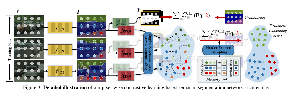
七、Pixel Contrast Cross Entropy Loss

论文：Exploring Cross-Image Pixel Contrast for Semantic Segmentation

自己使用paddlepaddle复现的地址（仅实现BatchSample）：contrast_seg_paddle

Pixel Contrast Cross Entropy Loss并不是设计应对数据不平衡问题，但是它的样本采样策略在一定程度上可以应对数据不平衡问题，可作为辅助损失函数使用。

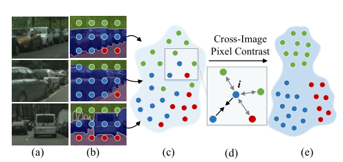
对于语义分割任务，当考虑上下文信息时一般是指的图片的上下文信息，但是本文作者提出利用”全局”（数据集所有图片）上下文信息来提升语义分割效果。核心思想在于：对于数据集中所有的同类像素，它的embedding应该是相似的，对于不同类别的像素，它的embedding应该是不同的。于是作者提出Pixel Contrast Cross Entropy Loss，目标是使同类像素的embedding尽可能靠近，不同类别像素的embedding尽可能远离。

如下图，对不同图片中的同类像素，通过对比学习的方法使同类像素的embedding靠近，不同类别像素的embedding远离，来提升语义分割的效果。

网络结构

对于一个任意的语义分割网络，额外引入一个project，project输出像素对应的embedding，将embedding送入Pixel Contrast Cross Entropy Loss优化，提高语义分割的效果。（相当于引入了一个辅助损失函数）

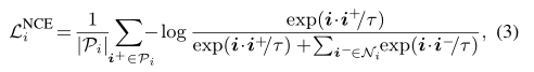
对比损失

得到了embedding，需要设计一个损失函数，该损失函数实现的功能为：使相同类别的embedding尽可能靠近，不同类别的embedding尽可能远离。怎么通过衡量2个embedding的距离呢？通过点积运算，2个向量点积值越大，表示越相似，越小表示越不相似。

损失函数如下式，

表示embedding向量，表示与同类别的embedding向量，表示点积运算，和相似性越低，损失函数越接近0，相似度越高，损失越大。

需要注意的是：embedding不是采集自一张图片，而是采集自不同图片

采样策略

首先给出困难样本的定义：

接近于-1，则为正困难样本（理想状态接近1），若接近1，则 为负困难样本（理想状态为1）。

文中提出3种采样策略来选择训练样本：

1、 Hardest Example Sampling

从正困难样本和负困难样本中各自挑选最难的K个样本参与训练。

2、 Semi-Hard Example Sampling

对于embedding向量

，选择与其最近的10%个负样本（负困难样本）和最远的10%个正样本（正困难样本）构成集合，每次训练从集合中挑选K个样本参与训练。

3、Segmentation-Aware Hard Anchor Sampling

预测结果（使seg头的输出，不是project的输出）正确的像素对应的embedding作为易分类样本，预测结果错误的embedding作为难分类样本，每次训练从难分类样本和易分类样本中各随机挑选K个样本参与训练。

挑选样本的时候，为什么要一半难样本一半易样本？

如果只挑选困难样本进行分类，那么网络训练出来的分类器可能如下图：

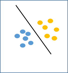
但是如果考虑到易样本呢？就可能变成这样了：

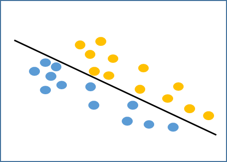
所以挑选样本的时候，从困难样本和容易的样本中各挑选一半。

声明

本篇文章禁止转载。

Original: https://blog.csdn.net/qq_40035462/article/details/123448323
Author: 嘟嘟太菜了
Title: 【语义分割】类别不平衡损失函数合集