

【Matlab 六自由度机器人】求运动学逆解
往期回顾
【汇总】
相关资源:
【Matlab 六自由度机器人】系列文章汇总 \fcolorbox{green}{aqua}{【Matlab 六自由度机器人】系列文章汇总 }【M a t l a b 六自由度机器人】系列文章汇总
【主线】
【补充说明】
- 关于灵活工作空间与可达工作空间的理解
- 关于改进型D-H参数(modified Denavit-Hartenberg)的详细建立步骤
- 关于旋转的参数化(欧拉角、姿态角、四元数)的相关问题
- 关于双变量函数atan2(x,y)的解释
- 关于机器人运动学反解的有关问题
前言
本篇介绍机器人逆运动学及逆解的求解方法,首先介绍如何理解逆向运动学,并利用D-H参数及正向运动学的齐次变换矩阵对机器人运动学逆解进行求解。
在博主读研期间,刚开始对机器人运动学逆解不甚了解,但在经历一次自己完全去钻研、尝试,独立写出属于自己的运动学逆解后,对机器人的结构有更加深刻的理解。因此希望初学机器人的朋友们也能够尝试独立去编写、尝试出自己的逆解代码,我相信,当你看到逆解解出的角度完全符合预期,也能够产生相当的成就感。
下面是运动学逆解的正文内容,主要讲述运动学逆解的方式和公式推算,最后进行代码的实现。
正文
一、运动学逆解
首先我们已经建立起了一个六自由度的机器人,在 D-H 参数 及机器人的 期望位姿 已知的情况下,求解机器人满足该期望位姿的各个关节变量,这种求解过程叫做机器人运动学逆解过程。求解机器人的逆运动学解法分为封闭解法和数值解法两种,其中封闭解法是指具有解析形式的解法,其求解速度比数值解法更快。
本文所研究的六自由度机器人,是具有六个旋转关节的串联型六自由度机器人,即RRR型的机器人。六自由度机器人的逆解封闭解法具体又可分为代数解法和几何解法,代数解法推导解析解的过程复杂,运算量较大,几何解法根据直观的几何关系获得关节变量的解析表达式,计算量较小。
本文主要讲解两种机器人运动学逆解的两种方法:
1. Pieper法
2. 常规法
1. Pieper 法
根据Pieper’s Solution的研究,如果六自由度机器人具有三个连续的轴交在同一点的情况,则手臂具有解析解。即六个关节均为旋转关节且后三个关节轴相交于一点的串联型机器人,其逆解具有封闭解。可以通过如下代数解法求解逆运动学的封闭解,该解法称为”三轴相交的 Pieper 解法”。下面进行各轴转角角度的公式推导。
我们知道,当后3个关节轴相交时,连杆坐标系 { 4 } , { 5 } , { 6 } {4},{5},{6}{4 },{5 },{6 } 的原点位于该交点,该交点在基坐标系 { 0 } {0}{0 } 中的坐标如下:
0 P 4 = 0 T 1 2 T 3 2 T 3 P 4 = [ x y z 1 ] T { }^{0} \boldsymbol{P}{4}={ }^{0} \boldsymbol{T}^{1}{ }{2} \boldsymbol{T}{3}^{2} \boldsymbol{T}^{3} \boldsymbol{P}{4}=\left[\begin{array}{llll} x & y & z & 1 \end{array}\right]^{\mathrm{T}}0 P 4 =0 T 1 2 T 3 2 T 3 P 4 =[x y z 1 ]T
对于齐次变换矩阵的变换通式的理解请参阅【Matlab 六自由度机器人】运动学正解(附MATLAB机器人正解完整代码)
由改进 _D-H_参数的连杆齐次变换矩阵式,应用齐次变换矩阵的变换通式
i − 1 T i = [ c o s θ i − s i n θ i 0 a i − 1 s i n θ i c o s α i − 1 c o s θ i c o s α i − 1 − s i n α i − 1 − s i n α i − 1 d i s i n θ i s i n α i − 1 c o s θ i s i n α i − 1 c o s α i − 1 c o s α i − 1 d i 0 0 0 1 ] ^{i-1}T_i =\left[ \begin{matrix} cosθ_i&-sinθ_i&0&a_{i-1} \ sinθ_icosα_{i-1}&cosθ_icosα_{i-1}&-sinα_{i-1}&-sinα_{i-1}d_{i} \ sinθ_isinα_{i-1}&cosθ_isinα_{i-1}&cosα_{i-1}&cosα_{i-1}d_{i} \ 0&0&0&1 \end{matrix} \right]i −1 T i =⎣⎢⎢⎡c o s θi s i n θi c o s αi −1 s i n θi s i n αi −1 0 −s i n θi c o s θi c o s αi −1 c o s θi s i n αi −1 0 0 −s i n αi −1 c o s αi −1 0 a i −1 −s i n αi −1 d i c o s αi −1 d i 1 ⎦⎥⎥⎤
可知当 i = 4 i=4 i =4 时,
0 P 4 = 1 0 T 2 1 T ( 3 2 T 3 P 4 ) = 1 0 T 2 1 T ( 3 2 T [ a 3 − d 4 s α 3 d 4 c α 3 1 ] ) = 1 0 T 2 1 T [ f 1 ( θ 3 ) f 2 ( θ 3 ) f 3 ( θ 3 ) 1 ] { }^{0} \boldsymbol{P}{4}={ }{1}^{0} \boldsymbol{T}{ }{2}^{1} \boldsymbol{T}\left({ }{3}^{2} \boldsymbol{T}^{3} \boldsymbol{P}{4}\right)={ }{1}^{0} \boldsymbol{T}{ }{2}^{1} \boldsymbol{T}\left({ }{3}^{2} \boldsymbol{T}\left[\begin{array}{c} a_{3} \ -d_{4} s \alpha_{3} \ d_{4} c \alpha_{3} \ 1 \end{array}\right]\right)={ }{1}^{0} \boldsymbol{T}{ }{2}^{1} \boldsymbol{T}\left[\begin{array}{c} f_{1}\left(\theta_{3}\right) \ f_{2}\left(\theta_{3}\right) \ f_{3}\left(\theta_{3}\right) \ 1 \end{array}\right]0 P 4 =1 0 T 2 1 T (3 2 T 3 P 4 )=1 0 T 2 1 T ⎝⎜⎜⎛3 2 T ⎣⎢⎢⎡a 3 −d 4 s α3 d 4 c α3 1 ⎦⎥⎥⎤⎠⎟⎟⎞=1 0 T 2 1 T ⎣⎢⎢⎡f 1 (θ3 )f 2 (θ3 )f 3 (θ3 )1 ⎦⎥⎥⎤
应用齐次变换矩阵对于 3 2 T { }{3}^{2} \boldsymbol{T}3 2 T 可以得到 f i f{i}f i 的表达式:
f 1 = a 3 c 3 + d 4 s α 3 s 3 + a 2 f 2 = a 3 c α 2 s 3 − d 4 s α 3 c α 2 c 3 − d 4 s α 2 c α 3 − d 3 s α 2 f 3 = a 3 s α 2 s 3 − d 4 s α 3 s α 2 c 3 + d 4 c α 2 c α 3 + d 3 c α 2 \begin{aligned} &f_{1}=a_{3} c_{3}+d_{4} s \alpha_{3} s_{3}+a_{2} \ &f_{2}=a_{3} c \alpha_{2} s_{3}-d_{4} s \alpha_{3} c \alpha_{2} c_{3}-d_{4} s \alpha_{2} c \alpha_{3}-d_{3} s \alpha_{2} \ &f_{3}=a_{3} s \alpha_{2} s_{3}-d_{4} s \alpha_{3} s \alpha_{2} c_{3}+d_{4} c \alpha_{2} c \alpha_{3}+d_{3} c \alpha_{2} \end{aligned}f 1 =a 3 c 3 +d 4 s α3 s 3 +a 2 f 2 =a 3 c α2 s 3 −d 4 s α3 c α2 c 3 −d 4 s α2 c α3 −d 3 s α2 f 3 =a 3 s α2 s 3 −d 4 s α3 s α2 c 3 +d 4 c α2 c α3 +d 3 c α2
对 1 0 T { }{1}^{0} \boldsymbol{T}1 0 T 和 2 1 T { }{2}^{1} \boldsymbol{T}2 1 T 应用齐次变换矩阵得到
0 P 4 = [ c 1 g 1 − s 1 g 2 s 1 g 1 + c 1 g 2 g 3 1 ] T { }^{0} \boldsymbol{P}{4}=\left[\begin{array}{llll} c{1} g_{1}-s_{1} g_{2} & s_{1} g_{1}+c_{1} g_{2} & g_{3} & 1 \end{array}\right]^{\mathrm{T}}0 P 4 =[c 1 g 1 −s 1 g 2 s 1 g 1 +c 1 g 2 g 3 1 ]T
g 1 、 g 2 、 g 3 g_{1} 、 g_{2} 、 g_{3}g 1 、g 2 、g 3 计算过程如下:
g 1 = c 2 f 1 − s 2 f 2 + a 1 g 2 = s 2 c α 1 f 1 + c 2 c α 1 f 2 − s α 1 f 3 − d 2 s α 1 g 3 = s 2 s α 1 f 1 + c 2 s α 1 f 2 + c α 1 f 3 + d 2 c α 1 \begin{aligned} &g_{1}=c_{2} f_{1}-s_{2} f_{2}+a_{1} \ &g_{2}=s_{2} c \alpha_{1} f_{1}+c_{2} c \alpha_{1} f_{2}-s \alpha_{1} f_{3}-d_{2} s \alpha_{1} \ &g_{3}=s_{2} s \alpha_{1} f_{1}+c_{2} s \alpha_{1} f_{2}+c \alpha_{1} f_{3}+d_{2} c \alpha_{1} \end{aligned}g 1 =c 2 f 1 −s 2 f 2 +a 1 g 2 =s 2 c α1 f 1 +c 2 c α1 f 2 −s α1 f 3 −d 2 s α1 g 3 =s 2 s α1 f 1 +c 2 s α1 f 2 +c α1 f 3 +d 2 c α1
令 r = x 2 + y 2 + z 2 r=x^{2}+y^{2}+z^{2}r =x 2 +y 2 +z 2,由上式可知
r = g 1 2 + g 2 2 + g 2 2 = f 1 2 + f 2 2 + f 2 2 + a 1 2 + d 2 2 + 2 d 2 f 3 + 2 a 1 ( c 2 f 1 − s 2 f 2 ) \begin{aligned} r &=g_{1}^{2}+g_{2}^{2}+g_{2}^{2} \ &=f_{1}^{2}+f_{2}^{2}+f_{2}^{2}+a_{1}^{2}+d_{2}^{2}+2 d_{2} f_{3}+2 a_{1}\left(c_{2} f_{1}-s_{2} f_{2}\right) \end{aligned}r =g 1 2 +g 2 2 +g 2 2 =f 1 2 +f 2 2 +f 2 2 +a 1 2 +d 2 2 +2 d 2 f 3 +2 a 1 (c 2 f 1 −s 2 f 2 )
由上式写出 Z \mathrm{Z}Z 轴分量的方程,可得系统的两个方程:
r = ( k 1 c 2 + k 2 s 2 ) 2 a 1 + k 3 z = ( k 1 s 2 − k 2 c 2 ) s α 2 + k 4 \begin{aligned} &r=\left(k_{1} c_{2}+k_{2} s_{2}\right) 2 a_{1}+k_{3} \ &z=\left(k_{1} s_{2}-k_{2} c_{2}\right) s \alpha_{2}+k_{4} \end{aligned}r =(k 1 c 2 +k 2 s 2 )2 a 1 +k 3 z =(k 1 s 2 −k 2 c 2 )s α2 +k 4
对于k 1 、 k 2 、 k 3 、 k 4 k_{1} 、 k_{2} 、 k_{3} 、 k_{4}k 1 、k 2 、k 3 、k 4 ,其计算如下:
k 1 = f 1 k 2 = − f 2 k 3 = f 1 2 + f 2 2 + f 3 2 + a 1 2 + d 2 2 + 2 d 2 f 3 k 4 = f 3 c α 1 + d 2 c α 1 \begin{aligned} &k_{1}=f_{1} \ &k_{2}=-f_{2} \ &k_{3}=f_{1}^{2}+f_{2}^{2}+f_{3}^{2}+a_{1}^{2}+d_{2}^{2}+2 d_{2} f_{3} \ &k_{4}=f_{3} c \alpha_{1}+d_{2} c \alpha_{1} \end{aligned}k 1 =f 1 k 2 =−f 2 k 3 =f 1 2 +f 2 2 +f 3 2 +a 1 2 +d 2 2 +2 d 2 f 3 k 4 =f 3 c α1 +d 2 c α1
之后求解 θ 3 \theta_{3}θ3 ,分三种情况:
(1) 若 a 1 = 0 a_{1}=0 a 1 =0,则 r = k 3 r=k_{3}r =k 3 ,此时 r r r 已知。 k 3 k_{3}k 3 的右边是关于 θ 3 \theta_{3}θ3 的函数。代入下式后,由包含 tan ( θ 3 / 2 ) \tan \left(\theta_{3} / 2\right)tan (θ3 /2 ) 的一元二次方程可以解出 θ 3 \theta_{3}θ3 ;
u = tan θ 2 , cos θ = 1 − u 2 1 + u 2 , sin θ = 2 u 1 + u 2 u=\tan \frac{\theta}{2}, \cos \theta=\frac{1-u^{2}}{1+u^{2}}, \sin \theta=\frac{2 u}{1+u^{2}}u =tan 2 θ,cos θ=1 +u 2 1 −u 2 ,sin θ=1 +u 2 2 u
(2) 若 s α 1 = 0 s \alpha_{1}=0 s α1 =0,则 z = k 4 z=k_{4}z =k 4 ,此时 z z z 已知。代入上式后,利用上面的一元 二次方程解出θ 3 \theta_{3}θ3
(3) 否则,从式r = ( k 1 c 2 + k 2 s 2 ) 2 a 1 + k 3 z = ( k 1 s 2 − k 2 c 2 ) s α 2 + k 4 \begin{aligned} &r=\left(k_{1} c_{2}+k_{2} s_{2}\right) 2 a_{1}+k_{3} \ &z=\left(k_{1} s_{2}-k_{2} c_{2}\right) s \alpha_{2}+k_{4} \end{aligned}r =(k 1 c 2 +k 2 s 2 )2 a 1 +k 3 z =(k 1 s 2 −k 2 c 2 )s α2 +k 4 中消去 s 2 s_{2}s 2 和 c 2 c_{2}c 2 ,得到
( r − k 3 ) 2 4 a 1 2 + ( z − k 4 ) 2 s 2 α 1 = k 1 2 + k 2 2 \frac{\left(r-k_{3}\right)^{2}}{4 a_{1}^{2}}+\frac{\left(z-k_{4}\right)^{2}}{s^{2} \alpha_{1}}=k_{1}^{2}+k_{2}^{2}4 a 1 2 (r −k 3 )2 +s 2 α1 (z −k 4 )2 =k 1 2 +k 2 2
代入u = tan θ 2 , cos θ = 1 − u 2 1 + u 2 , sin θ = 2 u 1 + u 2 u=\tan \frac{\theta}{2}, \cos \theta=\frac{1-u^{2}}{1+u^{2}}, \sin \theta=\frac{2 u}{1+u^{2}}u =tan 2 θ,cos θ=1 +u 2 1 −u 2 ,sin θ=1 +u 2 2 u 解出 θ 3 \theta_{3}θ3 后,可得到一个一元四次方程,由此可解出 θ 3 \theta_{3}θ3 。 解出 θ 3 \theta_{3}θ3 后,再解出 θ 2 \theta_{2}θ2 ,再根据0 P 4 = [ c 1 g 1 − s 1 g 2 s 1 g 1 + c 1 g 2 g 3 1 ] T { }^{0} \boldsymbol{P}{4}=\left[\begin{array}{llll} c{1} g_{1}-s_{1} g_{2} & s_{1} g_{1}+c_{1} g_{2} & g_{3} & 1 \end{array}\right]^{\mathrm{T}}0 P 4 =[c 1 g 1 −s 1 g 2 s 1 g 1 +c 1 g 2 g 3 1 ]T解出 θ 1 \theta_{1}θ1 。
Pieper 解法求解出了前三轴的关节变量,该解通常具有4组解或8组。由于后三轴的关节角只影响工具坐标系的方位,因此可以通过欧拉角解法求出后三轴的关节变量。
六自由度机器人工具坐标系的姿态,可以使用一组欧拉角( ψ , θ , φ ) (\psi, \theta, \varphi)(ψ,θ,φ) 来表示,该转角序列表示绕 x x x 轴,y y y 轴和 z z z 轴的旋转序列:先绕 z z z 轴旋转 ψ \psi ψ 角,再绕新坐标系的 y y y 轴旋转 θ \theta θ 角,最后绕新坐标系 的 z z z 轴旋转 φ \varphi φ 角。欧拉角变换 Euler ( ψ , θ , φ ) (\psi, \theta, \varphi)(ψ,θ,φ) 可以通过三个旋转矩阵相乘表示
Euler ( ψ , θ , φ ) = Rot ( z , ψ ) Rot ( y , θ ) Rot ( z , φ ) = [ c ψ c θ c φ − s ψ s φ − c ψ c θ s φ − s ψ c φ c ψ s θ 0 s ψ c θ c φ + c ψ s φ − s ψ c θ s φ + c ψ c φ s ψ s θ 0 − s θ c φ s θ s φ c θ 0 0 0 0 1 ] \begin{aligned} \operatorname{Euler}(\psi, \theta, \varphi) &=\operatorname{Rot}(z, \psi) \operatorname{Rot}(y, \theta) \operatorname{Rot}(z, \varphi) \ &=\left[\begin{array}{cccc} c \psi c \theta c \varphi-s \psi s \varphi & -c \psi c \theta s \varphi-s \psi c \varphi & c \psi s \theta & 0 \ s \psi c \theta c \varphi+c \psi s \varphi & -s \psi c \theta s \varphi+c \psi c \varphi & s \psi s \theta & 0 \ -s \theta c \varphi & s \theta s \varphi & c \theta & 0 \ 0 & 0 & 0 & 1 \end{array}\right] \end{aligned}E u l e r (ψ,θ,φ)=R o t (z ,ψ)R o t (y ,θ)R o t (z ,φ)=⎣⎢⎢⎡c ψc θc φ−s ψs φs ψc θc φ+c ψs φ−s θc φ0 −c ψc θs φ−s ψc φ−s ψc θs φ+c ψc φs θs φ0 c ψs θs ψs θc θ0 0 0 0 1 ⎦⎥⎥⎤
如果已知一个表示任意旋转的齐次变换, 即已知姿态矩阵 R \boldsymbol{R}R
R = [ n x o x a x n y o y a y n z o z a z ] \boldsymbol{R}=\left[\begin{array}{lll} n_{x} & o_{x} & a_{x} \ n_{y} & o_{y} & a_{y} \ n_{z} & o_{z} & a_{z} \end{array}\right]R =⎣⎡n x n y n z o x o y o z a x a y a z ⎦⎤
则根据姿态矩阵 R \boldsymbol{R}R 可求出其对应的欧拉角:
ψ = atan 2 ( a x , a y ) + 18 0 ∘ θ = atan 2 ( c ψ a x + s ψ a y , a z ) φ = atan 2 ( − s ψ n x + c ψ n y , − s ψ o x + c ψ o y ) \begin{aligned} &\psi=\operatorname{atan} 2\left(a_{x}, a_{y}\right)+180^{\circ} \ &\theta=\operatorname{atan} 2\left(c \psi a_{x}+s \psi a_{y}, a_{z}\right) \ &\varphi=\operatorname{atan} 2\left(-s \psi n_{x}+c \psi n_{y},-s \psi o_{x}+c \psi o_{y}\right) \end{aligned}ψ=a t a n 2 (a x ,a y )+1 8 0 ∘θ=a t a n 2 (c ψa x +s ψa y ,a z )φ=a t a n 2 (−s ψn x +c ψn y ,−s ψo x +c ψo y )对于6R型六自由度机器人,已经求得前三轴的关节变量,即可求出齐次变换矩 阵 3 0 T { }{3}^{0} \boldsymbol{T}3 0 T
3 0 T = 1 0 T ( θ 1 ) 2 1 T ( θ 2 ) 3 2 T ( θ 3 ) { }{3}^{0} \boldsymbol{T}={ }{1}^{0} \boldsymbol{T}\left(\theta{1}\right){ }{2}^{1} \boldsymbol{T}\left(\theta{2}\right){ }{3}^{2} \boldsymbol{T}\left(\theta{3}\right)3 0 T =1 0 T (θ1 )2 1 T (θ2 )3 2 T (θ3 )假设建立欧拉角 Euler ( ψ , θ , φ ) (\psi, \theta, \varphi)(ψ,θ,φ) 的坐标系为 { E } {\mathrm{E}}{E },则从基座标系 { 0 } {0}{0 } 到坐标系 { E } {E}{E } 的齐次变换矩阵为:
E 0 T = 3 0 T Rot ( x , α 3 ) { }{E}^{0} \boldsymbol{T}={ }{3}^{0} \boldsymbol{T} \operatorname{Rot}\left(x, \alpha_{3}\right)E 0 T =3 0 T R o t (x ,α3 )式中,α 3 \alpha_{3}α3 一表示改进 DH参数表中的第四轴的连杆扭角。 欧拉角表示的资态矩阵的计算方法如式(2-21)所示:
R = E 0 R ∗ 6 T R \boldsymbol{R}={ }{\mathrm{E}}^{{ }{\mathrm{0}}} \boldsymbol{R}*{ }{6}^{\mathrm{T}} \boldsymbol{R}R =E 0 R ∗6 T R其中E 0 R T { }{E}^{0} R^{\mathrm{T}}E 0 R T 一表示齐次变换矩阵 E 0 T { }{E}^{0} \boldsymbol{T}E 0 T 中的旋转矩阵的转置;6 0 R { }{6}^{0} R 6 0 R 一表示齐次变换矩阵 6 0 T { }_{6}^{0} \boldsymbol{T}6 0 T 中的旋转矩阵。
求出欧拉角姿态矩阵后,可通过ψ = atan 2 ( a x , a y ) + 18 0 ∘ θ = atan 2 ( c ψ a x + s ψ a y , a z ) φ = atan 2 ( − s ψ n x + c ψ n y , − s ψ o x + c ψ o y ) \begin{aligned} &\psi=\operatorname{atan} 2\left(a_{x}, a_{y}\right)+180^{\circ} \ &\theta=\operatorname{atan} 2\left(c \psi a_{x}+s \psi a_{y}, a_{z}\right) \ &\varphi=\operatorname{atan} 2\left(-s \psi n_{x}+c \psi n_{y},-s \psi o_{x}+c \psi o_{y}\right) \end{aligned}ψ=a t a n 2 (a x ,a y )+1 8 0 ∘θ=a t a n 2 (c ψa x +s ψa y ,a z )φ=a t a n 2 (−s ψn x +c ψn y ,−s ψo x +c ψo y )求出相应的欧拉角。所求得的欧 拉角与后三轴的关苖变量的关系为:
θ 4 = ψ , θ 5 = − θ , θ 6 = φ \theta_{4}=\psi, \theta_{5}=-\theta, \theta_{6}=\varphi θ4 =ψ,θ5 =−θ,θ6 =φ
由于机器人腕关节翻转,可以得到后三轴的另外一组解:
θ 4 ′ = θ 4 + 18 0 ∘ , θ 5 ′ = − θ 5 , θ 6 ′ = θ 6 + 18 0 ∘ \theta_{4}^{\prime}=\theta_{4}+180^{\circ}, \theta_{5}^{\prime}=-\theta_{5}, \theta_{6}^{\prime}=\theta_{6}+180^{\circ}θ4 ′=θ4 +1 8 0 ∘,θ5 ′=−θ5 ,θ6 ′=θ6 +1 8 0 ∘
上述算法可计算出的多组解,根据关节运动范围的限制可以舍弃一部分解,在余下的有效解中,通常选择最接近机器人当前位姿的”最短行程解”。
2. 《机器人学》常规求解
在求解运动学逆解前,我们先掌握运动学正解的知识,具体过程请参阅:【Matlab 六自由度机器人】运动学正解(附MATLAB机器人正解完整代码)
如前所述,矩阵右式的元素,或为零,或为常数,或者为第i i i至第6 6 6个关节变量的函数。矩阵相等表明其对应元素分别相等,并可从每一矩阵方程得到12 12 1 2个方程式,每个方程式对应于4 4 4个矢量n , o , a , p n,o,a,p n ,o ,a ,p的每一分量。我们先以之前建立过的 六自由度机器人 为例来阐述这些方程的求解。
该机器人的运动方程(设为方程式1)如下:
0 T 6 = [ n x o x a x p x n y o y a y p y n x o x a z p z 0 0 0 1 ] = 0 T 1 ( θ 1 ) 1 T 2 ( θ 2 ) 2 T 3 ( θ 3 ) 3 T 4 ( θ 4 ) 4 T 5 ( θ 5 ) 5 T 6 ( θ 6 ) { }^{0} \boldsymbol{T}{6}=\left[\begin{array}{cccc} n{x} & o_{x} & a_{x} & p_{x} \ n_{y} & o_{y} & a_{y} & p_{y} \ n_{x} & o_{x} & a_{z} & p_{z} \ 0 & 0 & 0 & 1 \end{array}\right]={ }^{0} \boldsymbol{T}{1}\left(\theta{1}\right)^{1} \boldsymbol{T}{2}\left(\theta{2}\right)^{2} \boldsymbol{T}{3}\left(\theta{3}\right)^{3} \boldsymbol{T}{4}\left(\theta{4}\right)^{4} \boldsymbol{T}{5}\left(\theta{5}\right)^{5} \boldsymbol{T}{6}\left(\theta{6}\right)0 T 6 =⎣⎢⎢⎡n x n y n x 0 o x o y o x 0 a x a y a z 0 p x p y p z 1 ⎦⎥⎥⎤=0 T 1 (θ1 )1 T 2 (θ2 )2 T 3 (θ3 )3 T 4 (θ4 )4 T 5 (θ5 )5 T 6 (θ6 )末端连杆的位姿已经给定,即 n , o , a n,o,a n ,o ,a 和 p p p 为已知,则求关节变量 θ 1 , θ 2 , ⋯ , θ 6 \theta_{1}, \theta_{2}, \cdots, \theta_{6}θ1 ,θ2 ,⋯,θ6 的值称为运动反解。用末知的连杆逆变换左乘方程式1两边,把关节变量分离出来,从而求解。具体步骤如下:
- 求 θ 1 \theta_{1}θ1
可用逆变换 0 T 1 − 1 ( θ 1 ) { }^{0} \boldsymbol{T}{1}^{-1}\left(\theta{1}\right)0 T 1 −1 (θ1 ) 左乘方程式1两边
0 T 1 − 1 ( θ 1 ) 0 T 6 = 1 T 2 ( θ 2 ) 2 T 3 ( θ 3 ) 3 T 4 ( θ 4 ) 4 T 5 ( θ 5 ) 5 T 6 ( θ 6 ) { }^{0} \boldsymbol{T}{1}^{-1}\left(\theta{1}\right)^{0} \boldsymbol{T}{6}={ }^{1} \boldsymbol{T}{2}\left(\theta_{2}\right)^{2} \boldsymbol{T}{3}\left(\theta{3}\right)^{3} \boldsymbol{T}{4}\left(\theta{4}\right)^{4} \boldsymbol{T}{5}\left(\theta{5}\right)^{5} \boldsymbol{T}{6}\left(\theta{6}\right)0 T 1 −1 (θ1 )0 T 6 =1 T 2 (θ2 )2 T 3 (θ3 )3 T 4 (θ4 )4 T 5 (θ5 )5 T 6 (θ6 )
[ c 1 s 1 0 0 − s 1 c 1 0 0 0 0 1 0 0 0 0 1 ] [ n x o x a x p x n y o y a y p y n z o x a z p x 0 0 0 1 ] = 1 T 6 \left[\begin{array}{rrrr} c_{1} & s_{1} & 0 & 0 \ -s_{1} & c_{1} & 0 & 0 \ 0 & 0 & 1 & 0 \ 0 & 0 & 0 & 1 \end{array}\right]\left[\begin{array}{cccc} n_{x} & o_{x} & a_{x} & p_{x} \ n_{y} & o_{y} & a_{y} & p_{y} \ n_{z} & o_{x} & a_{z} & p_{x} \ 0 & 0 & 0 & 1 \end{array}\right]={ }^{1} \boldsymbol{T}{6}⎣⎢⎢⎡c 1 −s 1 0 0 s 1 c 1 0 0 0 0 1 0 0 0 0 1 ⎦⎥⎥⎤⎣⎢⎢⎡n x n y n z 0 o x o y o x 0 a x a y a z 0 p x p y p x 1 ⎦⎥⎥⎤=1 T 6
令上式矩阵方程两瑞的元素 ( 2 , 4 ) (2,4)(2 ,4 ) 对应相等,可得
− s 1 p x + c 1 p y = d 2 -s{1} p_{x}+c_{1} p_{y}=d_{2}−s 1 p x +c 1 p y =d 2
利用三角代换
p x = ρ cos ϕ ; p y = ρ sin ϕ p_{x}=\rho \cos \phi ; \quad p_{y}=\rho \sin \phi p x =ρcos ϕ;p y =ρsin ϕ
式中,ρ = p x 2 + p y 2 ; ϕ = atan2 ( p y , p x ) \rho=\sqrt{p_{x}^{2}+p_{y}^{2}} ; \phi=\operatorname{atan2}\left(p_{y}, p_{x}\right)ρ=p x 2 +p y 2 ;ϕ=a t a n 2 (p y ,p x ) ,通过代换得到 θ 1 \theta_{1}θ1 的解。
sin ( ϕ − θ 1 ) = d 2 / ρ ; cos ( ϕ − θ 1 ) = ± 1 − ( d 2 / ρ ) 2 ϕ − θ 1 = atan 2 [ d 2 ρ , ± 1 − ( d 2 ρ ) 2 ] θ 1 = atan 2 ( p y , p x ) − atan 2 ( d 2 , ± p x 2 + p y 2 − d 2 2 ) } \left.\begin{array}{l} \sin \left(\phi-\theta_{1}\right)=d_{2} / \rho ; \cos \left(\phi-\theta_{1}\right)=\pm \sqrt{1-\left(d_{2} / \rho\right)^{2}} \ \phi-\theta_{1}=\operatorname{atan} 2\left[\frac{d_{2}}{\rho}, \pm \sqrt{1-\left(\frac{d_{2}}{\rho}\right)^{2}}\right] \ \theta_{1}=\operatorname{atan} 2\left(p_{y}, p_{x}\right)-\operatorname{atan} 2\left(d_{2}, \pm \sqrt{p_{x}^{2}+p_{y}^{2}-d_{2}^{2}}\right) \end{array}\right}sin (ϕ−θ1 )=d 2 /ρ;cos (ϕ−θ1 )=±1 −(d 2 /ρ)2 ϕ−θ1 =a t a n 2 [ρd 2 ,±1 −(ρd 2 )2 ]θ1 =a t a n 2 (p y ,p x )−a t a n 2 (d 2 ,±p x 2 +p y 2 −d 2 2 )⎭⎪⎪⎪⎪⎪⎬⎪⎪⎪⎪⎪⎫
式中,正、负号对应于 θ 1 \theta_{1}θ1 的两个可能解。
- 求 θ 3 \theta_{3}θ3
在选定 θ 1 \theta_{1}θ1 的一个解之后,再令矩阵方程1 T 6 { }^{1} \boldsymbol{T}{6}1 T 6 两端的元素的 ( 1 , 4 ) (1,4)(1 ,4 ) 和 ( 3 , 4 ) (3,4)(3 ,4 ) 分别对应相等,即得两方程
c 1 p x + s 1 p y = a 3 c 23 − d 4 s 23 + a 2 c 2 − p x = a 3 s 23 + d 4 c 23 + a 2 s 2 } \left.\begin{array}{l} c{1} p_{x}+s_{1} p_{y}=a_{3} c_{23}-d_{4} s_{23}+a_{2} c_{2} \ -p_{x}=a_{3} s_{23}+d_{4} c_{23}+a_{2} s_{2} \end{array}\right}c 1 p x +s 1 p y =a 3 c 2 3 −d 4 s 2 3 +a 2 c 2 −p x =a 3 s 2 3 +d 4 c 2 3 +a 2 s 2 }
式− s 1 p x + c 1 p y = d 2 -s_{1} p_{x}+c_{1} p_{y}=d_{2}−s 1 p x +c 1 p y =d 2 与c 1 p x + s 1 p y = a 3 c 23 − d 4 s 23 + a 2 c 2 − p x = a 3 s 23 + d 4 c 23 + a 2 s 2 } \left.\begin{array}{l} c_{1} p_{x}+s_{1} p_{y}=a_{3} c_{23}-d_{4} s_{23}+a_{2} c_{2} \ -p_{x}=a_{3} s_{23}+d_{4} c_{23}+a_{2} s_{2} \end{array}\right}c 1 p x +s 1 p y =a 3 c 2 3 −d 4 s 2 3 +a 2 c 2 −p x =a 3 s 2 3 +d 4 c 2 3 +a 2 s 2 }的平方和为
a 3 c 3 − d 4 s 3 = k a_{3} c_{3}-d_{4} s_{3}=k a 3 c 3 −d 4 s 3 =k
式中,k = p x 2 + p y 2 + p x 2 − a 2 2 − a 3 2 − d 2 2 − d 4 2 2 a 2 k=\frac{p_{x}^{2}+p_{y}^{2}+p_{x}^{2}-a_{2}^{2}-a_{3}^{2}-d_{2}^{2}-d_{4}^{2}}{2 a_{2}}k =2 a 2 p x 2 +p y 2 +p x 2 −a 2 2 −a 3 2 −d 2 2 −d 4 2
方程a 3 c 3 − d 4 s 3 = k a_{3} c_{3}-d_{4} s_{3}=k a 3 c 3 −d 4 s 3 =k中已经消去 θ 2 \theta_{2}θ2 ,且方程a 3 c 3 − d 4 s 3 = k a_{3} c_{3}-d_{4} s_{3}=k a 3 c 3 −d 4 s 3 =k与− s 1 p x + c 1 p y = d 2 -s_{1} p_{x}+c_{1} p_{y}=d_{2}−s 1 p x +c 1 p y =d 2 具有相同形式,因而可由三角代换求解得到θ 3 \theta_{3}θ3
θ 3 = atan 2 ( a 3 , d 4 ) − atan 2 ( k , ± a 3 2 + d 4 2 − k 2 ) \theta_{3}=\operatorname{atan} 2\left(a_{3}, d_{4}\right)-\operatorname{atan} 2\left(k, \pm \sqrt{a_{3}^{2}+d_{4}^{2}-k^{2}}\right)θ3 =a t a n 2 (a 3 ,d 4 )−a t a n 2 (k ,±a 3 2 +d 4 2 −k 2 )
式中,正、负号对应 θ 3 \theta_{3}θ3 的两种可能解。
- 求 θ 2 \theta_{2}θ2
为求解 θ 2 \theta_{2}θ2 ,在矩阵方程1两边左乘逆变换 0 T 3 − 1 { }^{0} \boldsymbol{T}{3}^{-1}0 T 3 −1 。
[ 0 T 3 − 1 ( θ 1 , θ 2 , θ 3 ) 0 T 6 3 3 T 4 ( θ 4 ) 4 T 5 ( θ 5 ) 5 T 6 ( θ 6 ) − c 1 s 23 − s 1 s 23 − s 23 − a 23 c 3 − s 1 c 1 0 − a 2 s 3 0 0 0 1 ] [ n x o x a x p x n y o y a y p y n z v z a z p z 0 0 0 1 ] = 3 T 6 \left[\begin{array}{cccc} { }^{0} \boldsymbol{T}{3}^{-1}\left(\theta_{1}, \theta_{2}, \theta_{3}\right)^{0} \boldsymbol{T}{6} & { }^{3}{ }^{3} \boldsymbol{T}{4}\left(\theta_{4}\right){ }^{4} \boldsymbol{T}{5}\left(\theta{5}\right)^{5} \boldsymbol{T}{6}\left(\theta{6}\right) \ -c_{1} s_{23} & -s_{1} s_{23} & -s_{23} & -a_{23} c_{3} \ -s_{1} & c_{1} & 0 & -a_{2} s_{3} \ 0 & 0 & 0 & 1 \end{array}\right]\left[\begin{array}{cccc} n_{x} & o_{x} & a_{x} & p_{x} \ n_{y} & o_{y} & a_{y} & p_{y} \ n_{z} & v_{z} & a_{z} & p_{z} \ 0 & 0 & 0 & 1 \end{array}\right]={ }^{3} \boldsymbol{T}{6}⎣⎢⎢⎡0 T 3 −1 (θ1 ,θ2 ,θ3 )0 T 6 −c 1 s 2 3 −s 1 0 3 3 T 4 (θ4 )4 T 5 (θ5 )5 T 6 (θ6 )−s 1 s 2 3 c 1 0 −s 2 3 0 0 −a 2 3 c 3 −a 2 s 3 1 ⎦⎥⎥⎤⎣⎢⎢⎡n x n y n z 0 o x o y v z 0 a x a y a z 0 p x p y p z 1 ⎦⎥⎥⎤=3 T 6
式中,变换 3 T 6 { }^{3} \boldsymbol{T}{6}3 T 6 由正解出来的矩阵推出。令上式矩阵方程两边的元素 ( 1 , 4 ) (1,4)(1 ,4 ) 和 (2.4) 分别对应 相等可得
c 1 c 23 p x + s 1 c 23 p y − s 23 p z − a 2 c 3 = a 3 − c 1 s 23 p z − s 1 s 23 p y − c 23 p z + a 2 s 3 = d 4 } \left.\begin{array}{l} c_{1} c_{23} p_{x}+s_{1} c_{23} p_{y}-s_{23} p_{z}-a_{2} c_{3}=a_{3} \ -c_{1} s_{23} p_{z}-s_{1} s_{23} p_{y}-c_{23} p_{z}+a_{2} s_{3}=d_{4} \end{array}\right}c 1 c 2 3 p x +s 1 c 2 3 p y −s 2 3 p z −a 2 c 3 =a 3 −c 1 s 2 3 p z −s 1 s 2 3 p y −c 2 3 p z +a 2 s 3 =d 4 }联立求解得 s 23 s_{23}s 2 3 和 c 23 c_{23}c 2 3
{ s 23 = ( − a 3 − a 2 c 3 ) p z + ( c 1 p x + s 1 p y ) ( a 2 s 3 − d 4 ) p 2 2 + ( c 1 p x + s 1 p y ) 2 c 23 = ( − d 4 + a 2 s 3 ) p z − ( c 1 p x + s 1 p y ) ( − a 2 c 3 − a 4 ) p z 2 + ( c 1 p x + s 1 p y ) 2 \left{\begin{array}{l} s_{23}=\frac{\left(-a_{3}-a_{2} c_{3}\right) p_{z}+\left(c_{1} p_{x}+s_{1} p_{y}\right)\left(a_{2} s_{3}-d_{4}\right)}{p_{2}^{2}+\left(c_{1} p_{x}+s_{1} p_{y}\right)^{2}} \ c_{23}=\frac{\left(-d_{4}+a_{2} s_{3}\right) p_{z}-\left(c_{1} p_{x}+s_{1} p_{y}\right)\left(-a_{2} c_{3}-a_{4}\right)}{p_{z}^{2}+\left(c_{1} p_{x}+s_{1} p_{y}\right)^{2}} \end{array}\right.{s 2 3 =p 2 2 +(c 1 p x +s 1 p y )2 (−a 3 −a 2 c 3 )p z +(c 1 p x +s 1 p y )(a 2 s 3 −d 4 )c 2 3 =p z 2 +(c 1 p x +s 1 p y )2 (−d 4 +a 2 s 3 )p z −(c 1 p x +s 1 p y )(−a 2 c 3 −a 4 )
s 23 s_{23}s 2 3 和 c 23 c_{23}c 2 3 表达式的分母相等,且为正。于是θ 23 = θ 2 + θ 3 = atan2 [ − ( a 3 + a 2 c 3 ) p z + ( c 1 p x + s 1 p y ) ( a 2 s 3 − d 4 ) , ( − d 4 + a 2 s 3 ) p x + ( c 1 p x + s 1 p y ) ( a 2 c 3 + a 3 ) ] \begin{aligned} \theta_{23}=\theta_{2}+\theta_{3}=& \operatorname{atan2}\left[-\left(a_{3}+a_{2} c_{3}\right) p_{z}+\left(c_{1} p_{x}+s_{1} p_{y}\right)\left(a_{2} s_{3}-d_{4}\right),\left(-d_{4}+a_{2} s_{3}\right) p_{x}\right.\ &\left.+\left(c_{1} p_{x}+s_{1} p_{y}\right)\left(a_{2} c_{3}+a_{3}\right)\right] \end{aligned}θ2 3 =θ2 +θ3 =a t a n 2 [−(a 3 +a 2 c 3 )p z +(c 1 p x +s 1 p y )(a 2 s 3 −d 4 ),(−d 4 +a 2 s 3 )p x +(c 1 p x +s 1 p y )(a 2 c 3 +a 3 )]
根据 θ 1 \theta_{1}θ1 和 θ 3 \theta_{3}θ3 解的四种可能组合,由上式可以得到相应的四种可能值 θ 23 \theta_{23}θ2 3 ,于是可得到 θ 2 \theta_{2}θ2 的四种可能解
θ 2 = θ 23 − θ 3 \theta_{2}=\theta_{23}-\theta_{3}θ2 =θ2 3 −θ3
式中,θ 2 \theta_{2}θ2 取与 θ 3 \theta_{3}θ3 相对应的值。
- 求 θ 4 \theta_{4}θ4
因为式 (3.75) 的左边均为已知,令两边元素 ( 1 , 3 ) (1,3)(1 ,3 ) 和 ( 3 , 3 ) (3,3)(3 ,3 ) 分别对应相等,则可得
{ a x c 1 c 23 + a y s 1 c 23 − a x s 23 = − c 4 s 5 − a x s y + a y c 1 = s 4 s 5 \left{\begin{array}{l} a_{x} c_{1} c_{23}+a_{y} s_{1} c_{23}-a_{x} s_{23}=-c_{4} s_{5} \ -a_{x} s_{y}+a_{y} c_{1}=s_{4} s_{5} \end{array}\right.{a x c 1 c 2 3 +a y s 1 c 2 3 −a x s 2 3 =−c 4 s 5 −a x s y +a y c 1 =s 4 s 5
只要 s 5 ≠ 0 s_{5} \neq 0 s 5 =0,便可求出 θ 4 \theta_{4}θ4
θ 4 = atan 2 ( − a 4 s 1 + a y c 1 , − a x c 1 c 23 − a y s 1 c 23 + a x s 23 ) \theta_{4}=\operatorname{atan} 2\left(-a_{4} s_{1}+a_{y} c_{1},-a_{x} c_{1} c_{23}-a_{y} s_{1} c_{23}+a_{x} s_{23}\right)θ4 =a t a n 2 (−a 4 s 1 +a y c 1 ,−a x c 1 c 2 3 −a y s 1 c 2 3 +a x s 2 3 )
当 s 5 = 0 s_{5}=0 s 5 =0 时,机械手处于奇㫒形位。此时,关节轴 4 和 6 重合,只能解出 θ 4 \theta_{4}θ4 与 θ 6 \theta_{6}θ6 的和或 差。奇异形位可以由式 (3.79)中 atan 2 \operatorname{atan} 2 a t a n 2 的两个变量是否都接近零来判别。若都接近零,则为奇异形位,否则,不是奇异形位。在奇异形位时,可任意选取 θ 4 \theta_{4}θ4 的值,再计箅相应的 θ 6 \theta_{6}θ6 值。
- 求 θ 5 \theta_{5}θ5
据求出的 θ 4 \theta_{4}θ4 ,可进一步解出 θ 5 \theta_{5}θ5 ,将方程1两端左乘逆变换 0 T 4 ( θ 1 , θ 2 , θ 3 , θ 4 ) { }^{0} \boldsymbol{T}{4}{ }^{}\left(\theta{1}, \theta_{2}, \theta_{3}, \theta_{4}\right)0 T 4 (θ1 ,θ2 ,θ3 ,θ4 ),
0 T 4 − 1 ( θ 1 , θ 2 , θ 3 , θ 4 ) 0 T 6 = 4 T 5 ( θ 5 ) 5 T 6 ( θ 6 ) { }^{0} \boldsymbol{T}{4}^{-1}\left(\theta{1}, \theta_{2}, \theta_{3}, \theta_{4}\right){ }^{0} \boldsymbol{T}{6}={ }^{4} \boldsymbol{T}{5}\left(\theta_{5}\right)^{5} \boldsymbol{T}{6}\left(\theta{6}\right)0 T 4 −1 (θ1 ,θ2 ,θ3 ,θ4 )0 T 6 =4 T 5 (θ5 )5 T 6 (θ6 )
因下面方程式的左边 θ 1 , θ 2 , θ 3 \theta_{1}, \theta_{2}, \theta_{3}θ1 ,θ2 ,θ3 和 θ 4 \theta_{4}θ4 均已解出, 逆变换 0 T 4 − 1 ( θ 1 , θ 2 , θ 3 , θ 4 ) { }^{0} T_{4}^{-1}\left(\theta_{1}, \theta_{2}, \theta_{3}, \theta_{4}\right)0 T 4 −1 (θ1 ,θ2 ,θ3 ,θ4 ) 为
[ c 1 c 23 c 4 + s 1 s 4 s 1 c 23 c 4 − c 1 s 4 − s 23 c 4 − a 2 c 3 c 4 + d 2 s 4 − a 3 c 4 − c 1 c 23 s 4 + s 1 c 4 − s 1 c 23 s 4 − c 1 c 4 s 23 s 4 a 2 c 3 s 4 + d 2 c 4 + a 3 s 4 − c 1 s 23 − s 1 s 23 − c 23 a 2 s 3 − d 4 0 0 0 1 ] \left[\begin{array}{cccc} c_{1} c_{23} c_{4}+s_{1} s_{4} & s_{1} c_{23} c_{4}-c_{1} s_{4} & -s_{23} c_{4} & -a_{2} c_{3} c_{4}+d_{2} s_{4}-a_{3} c_{4} \ -c_{1} c_{23} s_{4}+s_{1} c_{4} & -s_{1} c_{23} s_{4}-c_{1} c_{4} & s_{23} s_{4} & a_{2} c_{3} s_{4}+d_{2} c_{4}+a_{3} s_{4} \ -c_{1} s_{23} & -s_{1} s_{23} & -c_{23} & a_{2} s_{3}-d_{4} \ 0 & 0 & 0 & 1 \end{array}\right]⎣⎢⎢⎡c 1 c 2 3 c 4 +s 1 s 4 −c 1 c 2 3 s 4 +s 1 c 4 −c 1 s 2 3 0 s 1 c 2 3 c 4 −c 1 s 4 −s 1 c 2 3 s 4 −c 1 c 4 −s 1 s 2 3 0 −s 2 3 c 4 s 2 3 s 4 −c 2 3 0 −a 2 c 3 c 4 +d 2 s 4 −a 3 c 4 a 2 c 3 s 4 +d 2 c 4 +a 3 s 4 a 2 s 3 −d 4 1 ⎦⎥⎥⎤
上式方程式的右边 4 T 6 ( θ 5 , θ 6 ) = 4 T 5 ( θ 5 ) 5 T 6 ( θ 6 ) { }^{4} \boldsymbol{T}{6}\left(\theta{5}, \theta_{6}\right)={ }^{4} \boldsymbol{T}{5 } \left(\theta{5}\right){ }^{5} \boldsymbol{T}{6}\left(\theta{6}\right)4 T 6 (θ5 ,θ6 )=4 T 5 (θ5 )5 T 6 (θ6 ),由正解得到的4 T 6 { }^{4} \boldsymbol{T}{6}4 T 6 给出。据矩阵两边元素 ( 1 , 3 ) (1,3)(1 ,3 ) 和 ( 3 , 3 ) (3,3)(3 ,3 ) 分别对应相等,可得
a x ( c 1 c 23 c 4 + s 1 s 4 ) + a y ( s 1 c 23 c 4 − c 1 s 4 ) − a z ( s 23 c 4 ) = − s 5 a x ( − c 1 s 23 ) + a y ( − s i s 23 ) + a z ( − c 23 ) = c 5 } \left.\begin{array}{l} a{x}\left(c_{1} c_{23} c_{4}+s_{1} s_{4}\right)+a_{y}\left(s_{1} c_{23} c_{4}-c_{1} s_{4}\right)-a_{z}\left(s_{23} c_{4}\right)&=-s_{5} \ a_{x}\left(-c_{1} s_{23}\right)+a_{y}\left(-s_{i} s_{23}\right)+a_{z}\left(-c_{23}\right)&=c_{5} \end{array}\right}a x (c 1 c 2 3 c 4 +s 1 s 4 )+a y (s 1 c 2 3 c 4 −c 1 s 4 )−a z (s 2 3 c 4 )a x (−c 1 s 2 3 )+a y (−s i s 2 3 )+a z (−c 2 3 )=−s 5 =c 5 }
由此得到 θ 5 \theta_{5}θ5 的封闭解
θ 5 = atan 2 ( s 5 , c 5 ) \theta_{5}=\operatorname{atan} 2\left(s_{5}, c_{5}\right)θ5 =a t a n 2 (s 5 ,c 5 )
- 求 θ 6 \theta_{6}θ6
将方程式1改写为
0 T 5 1 ( θ 1 , θ 2 , ⋯ , θ 5 ) 0 T 6 = 5 T 6 ( θ 6 ) { }^{0} \boldsymbol{T}{5}{ }^{1}\left(\theta{1}, \theta_{2}, \cdots, \theta_{5}\right)^{0} \boldsymbol{T}{6}={ }^{5} \boldsymbol{T}{6}\left(\theta_{6}\right)0 T 5 1 (θ1 ,θ2 ,⋯,θ5 )0 T 6 =5 T 6 (θ6 )
令上式的矩阵方程两边元素 ( 3 , 1 ) (3,1)(3 ,1 ) 和 ( 1 , 1 ) (1,1)(1 ,1 ) 分别对应相等,可得
− n x ( c 1 c 23 s 4 − s 1 c 4 ) − n y ( s 1 c 23 s 4 + c 1 c 4 ) + n z ( s 23 s 4 ) = s 6 n z [ ( c 1 c 23 c + + s 1 s 4 ) c 5 − c s 23 s 5 ] + n y [ ( s 1 c 23 c 4 − c 1 s 4 ) c 5 − s 1 s 23 s 5 ] − n z ( s 23 c 4 c 5 + c 23 s 5 ) = c 6 \begin{aligned} -n_{x}\left(c_{1} c_{23} s_{4}-s_{1} c_{4}\right)-n_{y}\left(s_{1} c_{23} s_{4}+c_{1} c_{4}\right)+n_{z}\left(s_{23} s_{4}\right)&=s_{6} \ n_{z}\left[\left(c_{1} c_{23} c_{+}+s_{1} s_{4}\right) c_{5}-c s_{23} s_{5}\right]+n_{y}\left[\left(s_{1} c_{23} c_{4}-c_{1} s_{4}\right) c_{5}-s_{1} s_{23} s_{5}\right] &-n_{z}\left(s_{23} c_{4} c_{5}+c_{23} s_{5}\right)&=c_{6} \end{aligned}−n x (c 1 c 2 3 s 4 −s 1 c 4 )−n y (s 1 c 2 3 s 4 +c 1 c 4 )+n z (s 2 3 s 4 )n z [(c 1 c 2 3 c ++s 1 s 4 )c 5 −c s 2 3 s 5 ]+n y [(s 1 c 2 3 c 4 −c 1 s 4 )c 5 −s 1 s 2 3 s 5 ]=s 6 −n z (s 2 3 c 4 c 5 +c 2 3 s 5 )=c 6
从而可求出 θ 6 \theta_{6}θ6 的封闭解
θ 6 = atan 2 ( s 6 , c 6 ) \theta_{6}=\operatorname{atan} 2\left(s_{6}, c_{6}\right)θ6 =a t a n 2 (s 6 ,c 6 )六自由度机器人的运动学反解可能存在8 8 8种解。但是,由于结构的限制,例如各关节变量不 能在全部 36 0 ∘ 360^{\circ}3 6 0 ∘ 范围内运动,有些解不能实现。在机器人存在多种解的情况下,应选取其中满意的一组解,以满足机器人的工作要求。
后续更新简单理解的步骤
二、代码实现
1. 机器人模型的建立
根据往期文章,对六自由度机器人具体建模方法可参阅以下文章:
2. Pieper 法求六自由度机器人逆解
建立好机器人模型后,已知期望位姿的矩阵a a a。将所求解的机器人的模型放入逆解脚本中,脚本的输入为期望位姿矩阵a a a,输出为角度J J J
代码如下:
function [J] = MODikine(a)
%% MOD-DH参数
%定义连杆的D-H参数
%连杆偏移
d1 = 398;
d2 = -0.299;
d3 = 0;
d4 = 556.925;
d5 = 0;
d6 = 165;
%连杆长度
a1 = 0;
a2 = 168.3;
a3 = 650.979;
a4 = 156.240;
a5 = 0;
a6 = 0;
%连杆扭角
alpha1 = 0;
alpha2 = pi/2;
alpha3 = 0;
alpha4 = pi/2;
alpha5 = -pi/2;
alpha6 = pi/2;

%%
nx=a(1,1);ox=a(1,2);ax=a(1,3);px=a(1,4);
ny=a(2,1);oy=a(2,2);ay=a(2,3);py=a(2,4);
nz=a(3,1);oz=a(3,2);az=a(3,3);pz=a(3,4);

% 求解关节角1
    theta1_1 = atan2(py,px)-atan2(d2,sqrt(px^2+py^2-d2^2));
    theta1_2 = atan2(py,px)-atan2(d2,-sqrt(px^2+py^2-d2^2));

% 求解关节角3
    m3_1 = (px^2+py^2+pz^2-a2^2-a3^2-d2^2-d4^2)/(2*a2);
    theta3_1 = atan2(a3,d4)-atan2(m3_1,sqrt(a3^2+d4^2-m3_1^2));
    theta3_2 = atan2(a3,d4)-atan2(m3_1,-sqrt(a3^2+d4^2-m3_1^2));

% 求解关节角2
    ms2_1 = -((a3+a2*cos(theta3_1))*pz)+(cos(theta1_1)*px+sin(theta1_1)*py)*(a2*sin(theta3_1)-d4);
    mc2_1 = (-d4+a2*sin(theta3_1))*pz+(cos(theta1_1)*px+sin(theta1_1)*py)*(a2*cos(theta3_1)+a3);
    theta23_1 = atan2(ms2_1,mc2_1);
    theta2_1 = theta23_1 - theta3_1;

    ms2_2 = -((a3+a2*cos(theta3_1))*pz)+(cos(theta1_2)*px+sin(theta1_2)*py)*(a2*sin(theta3_1)-d4);
    mc2_2 = (-d4+a2*sin(theta3_1))*pz+(cos(theta1_2)*px+sin(theta1_2)*py)*(a2*cos(theta3_1)+a3);
    theta23_2 = atan2(ms2_2,mc2_2);
    theta2_2 = theta23_2 - theta3_1;

    ms2_3 = -((a3+a2*cos(theta3_2))*pz)+(cos(theta1_1)*px+sin(theta1_1)*py)*(a2*sin(theta3_2)-d4);
    mc2_3 = (-d4+a2*sin(theta3_2))*pz+(cos(theta1_1)*px+sin(theta1_1)*py)*(a2*cos(theta3_2)+a3);
    theta23_3 = atan2(ms2_3,mc2_3);
    theta2_3 = theta23_3 - theta3_2;

    ms2_4 = -((a3+a2*cos(theta3_2))*pz)+(cos(theta1_2)*px+sin(theta1_2)*py)*(a2*sin(theta3_2)-d4);
    mc2_4 = (-d4+a2*sin(theta3_2))*pz+(cos(theta1_2)*px+sin(theta1_2)*py)*(a2*cos(theta3_2)+a3);
    theta23_4 = atan2(ms2_4,mc2_4);
    theta2_4 = theta23_4 - theta3_2;

% 求解关节角4
    ms4_1=-ax*sin(theta1_1)+ay*cos(theta1_1);
    mc4_1=-ax*cos(theta1_1)*cos(theta23_1)-ay*sin(theta1_1)*cos(theta23_1)+az*sin(theta23_1);
    theta4_1=atan2(ms4_1,mc4_1);

    ms4_2=-ax*sin(theta1_2)+ay*cos(theta1_2);
    mc4_2=-ax*cos(theta1_2)*cos(theta23_2)-ay*sin(theta1_2)*cos(theta23_2)+az*sin(theta23_2);
    theta4_2=atan2(ms4_2,mc4_2);

    ms4_3=-ax*sin(theta1_1)+ay*cos(theta1_1);
    mc4_3=-ax*cos(theta1_1)*cos(theta23_3)-ay*sin(theta1_1)*cos(theta23_3)+az*sin(theta23_3);
    theta4_3=atan2(ms4_3,mc4_3);

    ms4_4=-ax*sin(theta1_2)+ay*cos(theta1_2);
    mc4_4=-ax*cos(theta1_2)*cos(theta23_4)-ay*sin(theta1_2)*cos(theta23_4)+az*sin(theta23_4);
    theta4_4=atan2(ms4_4,mc4_4);

% 求解关节角5
    ms5_1=-ax*(cos(theta1_1)*cos(theta23_1)*cos(theta4_1)+sin(theta1_1)*sin(theta4_1))-ay*(sin(theta1_1)*cos(theta23_1)*cos(theta4_1)-cos(theta1_1)*sin(theta4_1))+az*(sin(theta23_1)*cos(theta4_1));
    mc5_1= ax*(-cos(theta1_1)*sin(theta23_1))+ay*(-sin(theta1_1)*sin(theta23_1))+az*(-cos(theta23_1));
    theta5_1=atan2(ms5_1,mc5_1);

    ms5_2=-ax*(cos(theta1_2)*cos(theta23_2)*cos(theta4_2)+sin(theta1_2)*sin(theta4_2))-ay*(sin(theta1_2)*cos(theta23_2)*cos(theta4_2)-cos(theta1_2)*sin(theta4_2))+az*(sin(theta23_2)*cos(theta4_2));
    mc5_2= ax*(-cos(theta1_2)*sin(theta23_2))+ay*(-sin(theta1_2)*sin(theta23_2))+az*(-cos(theta23_2));
    theta5_2=atan2(ms5_2,mc5_2);

    ms5_3=-ax*(cos(theta1_1)*cos(theta23_3)*cos(theta4_3)+sin(theta1_1)*sin(theta4_3))-ay*(sin(theta1_1)*cos(theta23_3)*cos(theta4_3)-cos(theta1_1)*sin(theta4_3))+az*(sin(theta23_3)*cos(theta4_3));
    mc5_3= ax*(-cos(theta1_1)*sin(theta23_3))+ay*(-sin(theta1_1)*sin(theta23_3))+az*(-cos(theta23_3));
    theta5_3=atan2(ms5_3,mc5_3);

    ms5_4=-ax*(cos(theta1_2)*cos(theta23_4)*cos(theta4_4)+sin(theta1_2)*sin(theta4_4))-ay*(sin(theta1_2)*cos(theta23_4)*cos(theta4_4)-cos(theta1_2)*sin(theta4_4))+az*(sin(theta23_4)*cos(theta4_4));
    mc5_4= ax*(-cos(theta1_2)*sin(theta23_4))+ay*(-sin(theta1_2)*sin(theta23_4))+az*(-cos(theta23_4));
    theta5_4=atan2(ms5_4,mc5_4);

% 求解关节角6
    ms6_1=-nx*(cos(theta1_1)*cos(theta23_1)*sin(theta4_1)-sin(theta1_1)*cos(theta4_1))-ny*(sin(theta1_1)*cos(theta23_1)*sin(theta4_1)+cos(theta1_1)*cos(theta4_1))+nz*(sin(theta23_1)*sin(theta4_1));
    mc6_1= nx*(cos(theta1_1)*cos(theta23_1)*cos(theta4_1)+sin(theta1_1)*sin(theta4_1))*cos(theta5_1)-nx*cos(theta1_1)*sin(theta23_1)*sin(theta4_1)+ny*(sin(theta1_1)*cos(theta23_1)*cos(theta4_1)+cos(theta1_1)*sin(theta4_1))*cos(theta5_1)-ny*sin(theta1_1)*sin(theta23_1)*sin(theta5_1)-nz*(sin(theta23_1)*cos(theta4_1)*cos(theta5_1)+cos(theta23_1)*sin(theta5_1));
    theta6_1=atan2(ms6_1,mc6_1);

    ms6_2=-nx*(cos(theta1_2)*cos(theta23_2)*sin(theta4_2)-sin(theta1_2)*cos(theta4_2))-ny*(sin(theta1_2)*cos(theta23_2)*sin(theta4_2)+cos(theta1_2)*cos(theta4_2))+nz*(sin(theta23_2)*sin(theta4_2));
    mc6_2= nx*(cos(theta1_2)*cos(theta23_2)*cos(theta4_2)+sin(theta1_2)*sin(theta4_2))*cos(theta5_2)-nx*cos(theta1_2)*sin(theta23_2)*sin(theta4_2)+ny*(sin(theta1_2)*cos(theta23_2)*cos(theta4_2)+cos(theta1_2)*sin(theta4_2))*cos(theta5_2)-ny*sin(theta1_2)*sin(theta23_2)*sin(theta5_2)-nz*(sin(theta23_2)*cos(theta4_2)*cos(theta5_2)+cos(theta23_2)*sin(theta5_2));
    theta6_2=atan2(ms6_2,mc6_2);

    ms6_3=-nx*(cos(theta1_1)*cos(theta23_3)*sin(theta4_3)-sin(theta1_1)*cos(theta4_3))-ny*(sin(theta1_1)*cos(theta23_3)*sin(theta4_3)+cos(theta1_1)*cos(theta4_3))+nz*(sin(theta23_3)*sin(theta4_3));
    mc6_3= nx*(cos(theta1_1)*cos(theta23_3)*cos(theta4_3)+sin(theta1_1)*sin(theta4_3))*cos(theta5_3)-nx*cos(theta1_1)*sin(theta23_3)*sin(theta4_3)+ny*(sin(theta1_1)*cos(theta23_3)*cos(theta4_3)+cos(theta1_1)*sin(theta4_3))*cos(theta5_3)-ny*sin(theta1_1)*sin(theta23_3)*sin(theta5_3)-nz*(sin(theta23_3)*cos(theta4_3)*cos(theta5_3)+cos(theta23_3)*sin(theta5_3));
    theta6_3=atan2(ms6_3,mc6_3);

    ms6_4=-nx*(cos(theta1_2)*cos(theta23_4)*sin(theta4_4)-sin(theta1_2)*cos(theta4_4))-ny*(sin(theta1_1)*cos(theta23_4)*sin(theta4_4)+cos(theta1_2)*cos(theta4_4))+nz*(sin(theta23_4)*sin(theta4_4));
    mc6_4= nx*(cos(theta1_2)*cos(theta23_4)*cos(theta4_4)+sin(theta1_2)*sin(theta4_4))*cos(theta5_4)-nx*cos(theta1_2)*sin(theta23_4)*sin(theta4_4)+ny*(sin(theta1_2)*cos(theta23_4)*cos(theta4_4)+cos(theta1_2)*sin(theta4_4))*cos(theta5_1)-ny*sin(theta1_2)*sin(theta23_4)*sin(theta5_4)-nz*(sin(theta23_4)*cos(theta4_4)*cos(theta5_4)+cos(theta23_4)*sin(theta5_4));
    theta6_4=atan2(ms6_4,mc6_4);

% 整理得到4组运动学非奇异逆解
theta_MOD1 = [
               theta1_1,theta2_1,theta3_1,theta4_1,theta5_1,theta6_1;
               theta1_2,theta2_2,theta3_1,theta4_2,theta5_2,theta6_2;
               theta1_1,theta2_3,theta3_2,theta4_3,theta5_3,theta6_3;
               theta1_2,theta2_4,theta3_2,theta4_4,theta5_4,theta6_4;
              ];
% 将操作关节'翻转'可得到另外4组解
theta_MOD2 = ...

    [
      theta1_1,theta2_1,theta3_1,theta4_1+pi,-theta5_1,theta6_1+pi;
      theta1_2,theta2_2,theta3_1,theta4_2+pi,-theta5_2,theta6_2+pi;
      theta1_1,theta2_3,theta3_2,theta4_3+pi,-theta5_3,theta6_3+pi;
      theta1_2,theta2_4,theta3_2,theta4_4+pi,-theta5_4,theta6_4+pi;
    ];

  J = [theta_MOD1;theta_MOD2];
end
3. 常规法求六自由度机器人逆解
由于自写的代码过长,阅读较为困难,因此贴上部分逆解代码过程。
建立好机器人模型后,已知期望位姿的矩阵a a a。将所求解的机器人的模型放入逆解脚本中,脚本的输入为期望位姿矩阵a a a,输出为角度J J J
这里的r o b o t robot r o b o t代表的是机器人的模型,a a a是已知的期望位姿的矩阵,输出是各轴的角度J J J
function [J] = Albert_MODikin(robot,a)
%% MOD-DH参数
%连杆偏移       %连杆长度       %连杆扭角
d1 = robot.d(1);a1 = robot.a(1);alpha1 = robot.alpha(1);
d2 = robot.d(2);a2 = robot.a(2);alpha2 = robot.alpha(2);
d3 = robot.d(3);a3 = robot.a(3);alpha3 = robot.alpha(3);
d4 = robot.d(4);a4 = robot.a(4);alpha4 = robot.alpha(4);
d5 = robot.d(5);a5 = robot.a(5);alpha5 = robot.alpha(5);
d6 = robot.d(6);a6 = robot.a(6);alpha6 = robot.alpha(6);

%%
nx=a(1,1);ox=a(1,2);ax=a(1,3);px=a(1,4);
ny=a(2,1);oy=a(2,2);ay=a(2,3);py=a(2,4);
nz=a(3,1);oz=a(3,2);az=a(3,3);pz=a(3,4);

%j1
j1a = py - ay*d6;
j1b = px - ax*d6;

j11 = atan2(j1a,j1b)-atan2(-d2, sqrt(j1a^2+j1b^2-d2^2));
j12 = atan2(j1a,j1b)-atan2(-d2,-sqrt(j1a^2+j1b^2-d2^2));

% 这部分是进行一个判断,将小于1e-16的数字看作0,建议删除。
if j11<1e-16
   j11 = 0;
end
if j12<1e-16
   j12 = 0;
end

%j3
j3a1 = px*cos(j11) - d6*(ax*cos(j11) + ay*sin(j11)) + py*sin(j11) - a2;
j3b1 = pz - d1 - az*d6;
j3k1 = j3a1^2 + j3b1^2 - a4^2 - d4^2 - a3^2;
j3d1 = j3k1/(2*a3);
j3a2 = px*cos(j12) - d6*(ax*cos(j12) + ay*sin(j12)) + py*sin(j12) - a2;
j3b2 = pz - d1 - az*d6;
j3k2 = j3a2^2 + j3b2^2 - a4^2 - d4^2 - a3^2;
j3d2 = j3k2/(2*a3);

j31 = atan2(j3d1, sqrt(abs(a4^2 + d4^2 - j3d1^2))) - atan2(a4,d4);%j11
j32 = atan2(j3d1,-sqrt(abs(a4^2 + d4^2 - j3d1^2))) - atan2(a4,d4);%j11
j33 = atan2(j3d2, sqrt(abs(a4^2 + d4^2 - j3d2^2))) - atan2(a4,d4);%j12
j34 = atan2(j3d2,-sqrt(abs(a4^2 + d4^2 - j3d2^2))) - atan2(a4,d4);%j12

% 经过一系列运算后,最终得到J
J = [j11 j21 j31 j41 j51 j61;
     j11 j22 j32 j42 j52 j62;
     j12 j23 j33 j43 j53 j63;
     j12 j24 j34 j44 j54 j64;
     j11 j21 j31 j45 j55 j65;
     j11 j22 j32 j46 j56 j66;
     j12 j23 j33 j47 j57 j67;
     j12 j24 j34 j48 j58 j68];

end
程序运行后的结果如下:
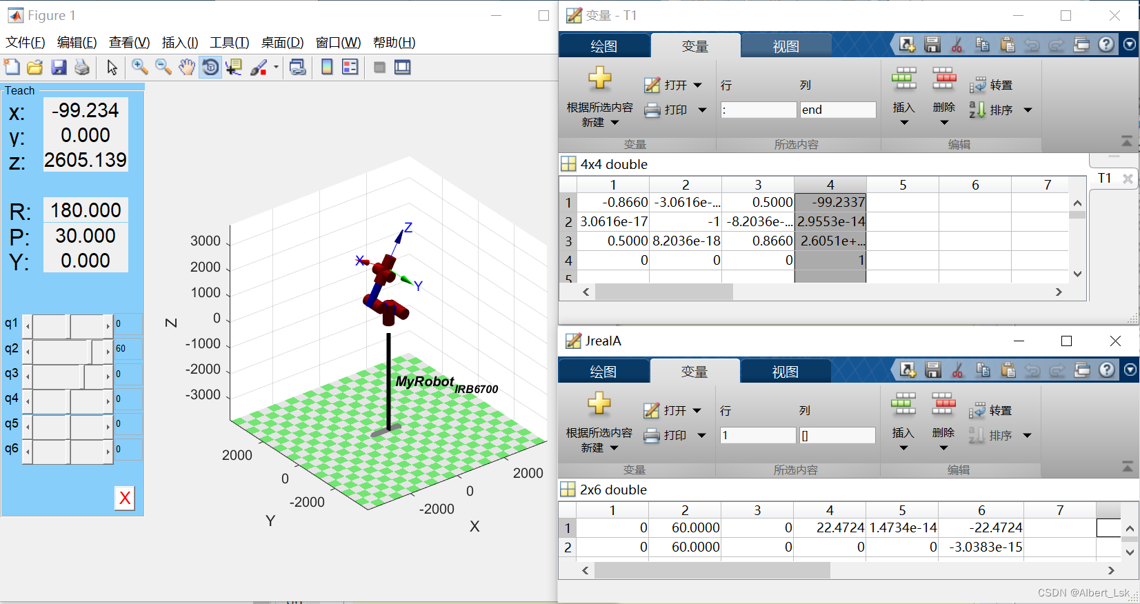

我们可以看到,左侧机器人示教器中,第二根轴的角度设为6 0 ∘ 60^{\circ}6 0 ∘,其位置矩阵为[ − 99.234 , 0 , 2605.139 ] [-99.234,0,2605.139][−9 9 .2 3 4 ,0 ,2 6 0 5 .1 3 9 ]。右上方正解的最后一列完全对应,右下方逆解得到的数值与输入的角度数一致,因此可知逆解程序完全可行。
总结
以上就是逆向运动学的内容,本文详细介绍了如何理解运动学逆解,以及对运动学逆解的求解方法的罗列及原理说明。最后对运动学逆解实现代码的编程,使逆解能够有效得到目标位姿所对应的各轴转角。
参考文献
- MATLAB机器人工具箱【1】——建模+正逆运动学+雅克比矩阵
- 六轴机器人matlab写运动学逆解函数(改进DH模型)
- 六轴机器人建模方法、正逆解、轨迹规划实例与Matalb Robotic Toolbox 的实现
Original: https://blog.csdn.net/AlbertDS/article/details/123679114
Author: Albert_Lsk
Title: 【Matlab 六自由度机器人】运动学逆解(附MATLAB机器人逆解代码)
原创文章受到原创版权保护。转载请注明出处:https://www.johngo689.com/646097/
转载文章受原作者版权保护。转载请注明原作者出处!