

目录
- 简介
- 10.2. 注意力汇聚:Nadaraya-Watson 核回归
* - 10.2.1. 生成数据集
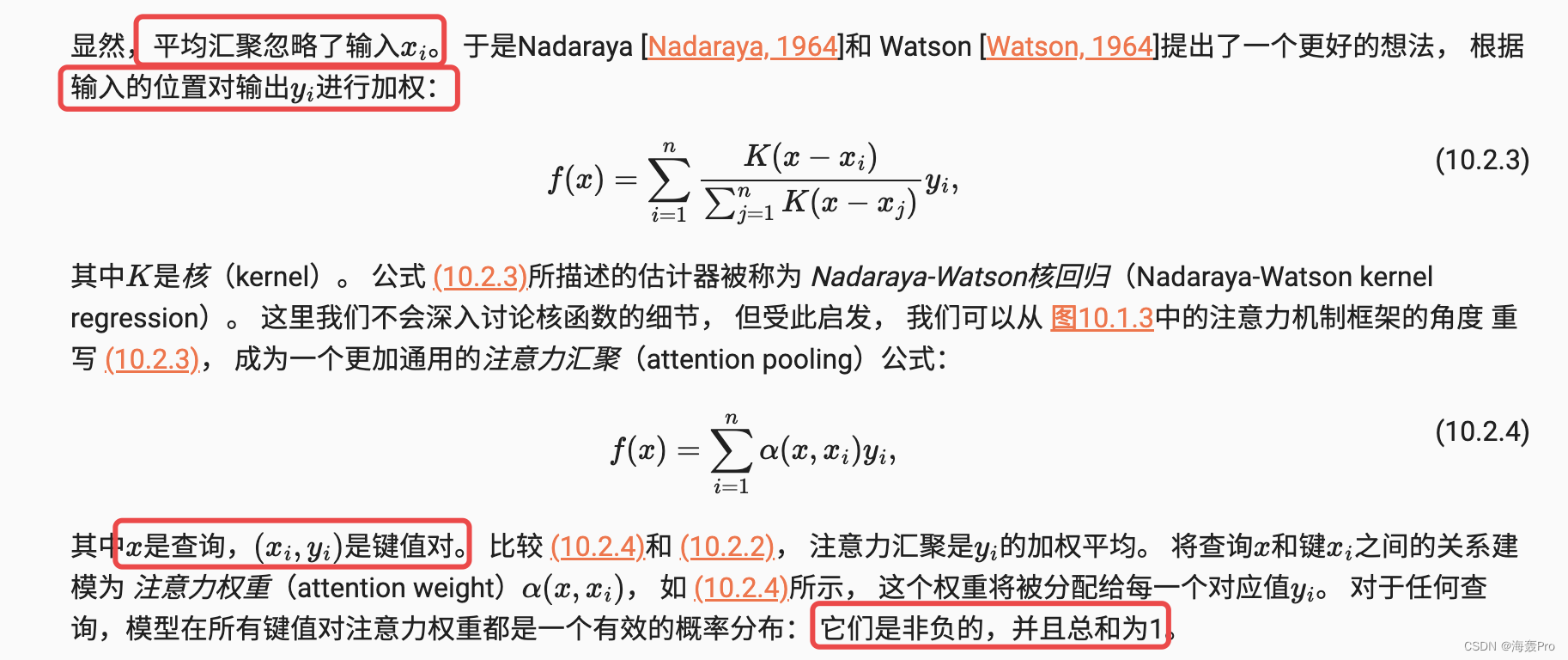
- 10.2.2. 平均汇聚
- 10.2.3. 非参数注意力汇聚
- 10.2.4. 带参数注意力汇聚
– - 10.2.5. 小结
- 结语


; 简介
Hello!
非常感谢您阅读海轰的文章,倘若文中有错误的地方,欢迎您指出~
ଘ(੭ˊᵕˋ)੭
昵称:海轰
标签:程序猿|C++选手|学生
简介:因C语言结识编程,随后转入计算机专业,获得过国家奖学金,有幸在竞赛中拿过一些国奖、省奖…已保研
学习经验:扎实基础 + 多做笔记 + 多敲代码 + 多思考 + 学好英语!
唯有努力💪
本文仅记录自己感兴趣的内容
10.2. 注意力汇聚:Nadaraya-Watson 核回归
在本节中,我们将介绍注 意力汇聚的更多细节, 以便从宏观上了解注意力机制在实践中的运作方式
具体来说,1964年提出的Nadaraya-Watson核回归模型 是一个简单但完整的例子,可以用于演示 具有注意力机制的机器学习
import torch
from torch import nn
from d2l import torch as d2l
10.2.1. 生成数据集

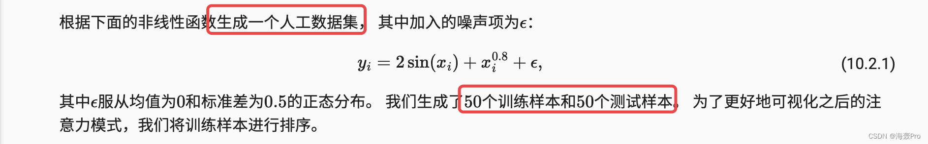
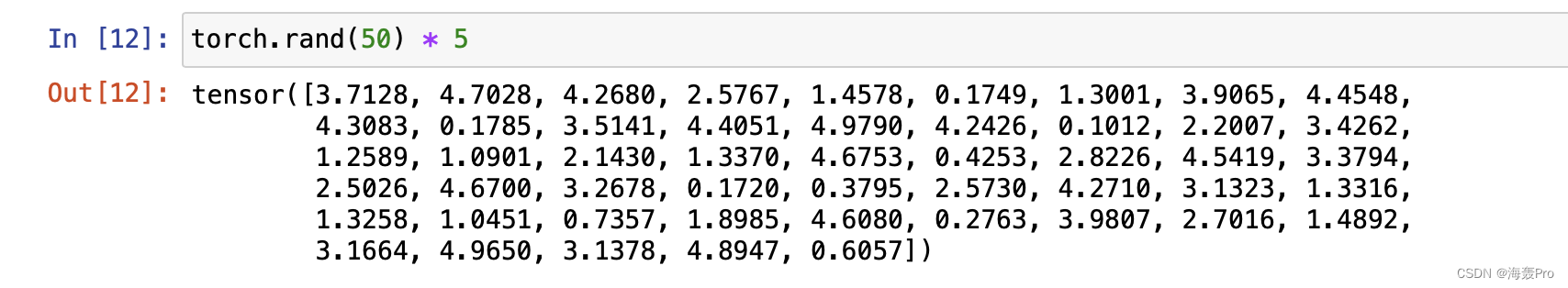
n_train = 50
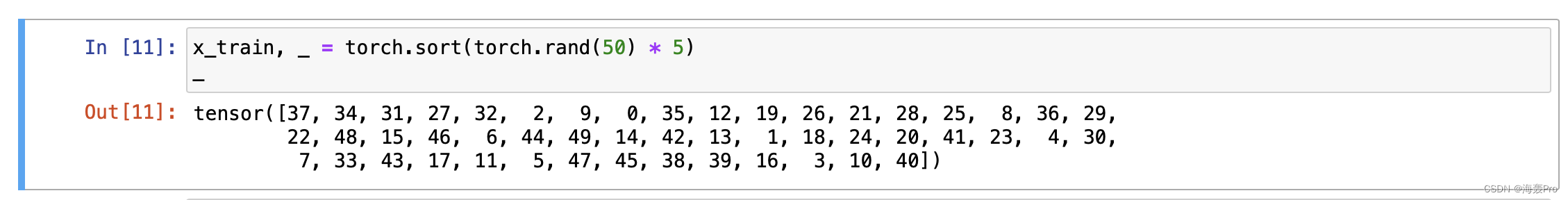
x_train, _ = torch.sort(torch.rand(n_train) * 5)
def f(x):
return 2 * torch.sin(x) + x**0.8
y_train = f(x_train) + torch.normal(0.0, 0.5, (n_train,))
x_test = torch.arange(0, 5, 0.1)
y_truth = f(x_test)
n_test = len(x_test)
n_test

Note

def plot_kernel_reg(y_hat):
    d2l.plot(x_test, [y_truth, y_hat], 'x', 'y', legend=['Truth', 'Pred'],
             xlim=[0, 5], ylim=[-1, 5])
    d2l.plt.plot(x_train, y_train, 'o', alpha=0.5);
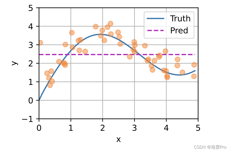
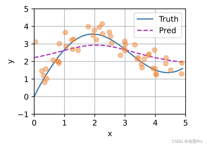
10.2.2. 平均汇聚
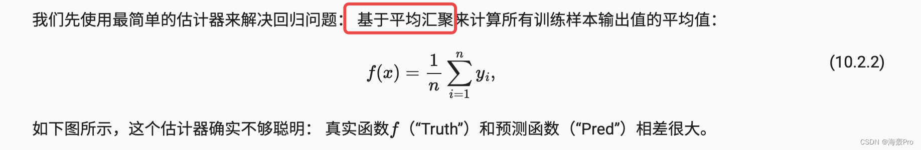
y_hat = torch.repeat_interleave(y_train.mean(), n_test)
plot_kernel_reg(y_hat)
10.2.3. 非参数注意力汇聚
Note
- 给定一个x x x(query)
- 首先计算x x x与x i x_i x i (key)之间的权重
- 然后利用这个权重 加权y i y_i y i (value)
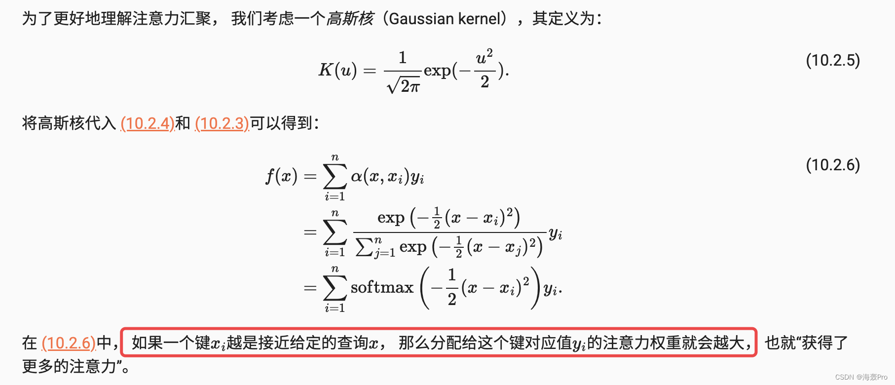
Note
- 这个高斯核可以理解为,利用x x x与x i x_i x i 计算y i y_i y i 应该分配的权重
Note
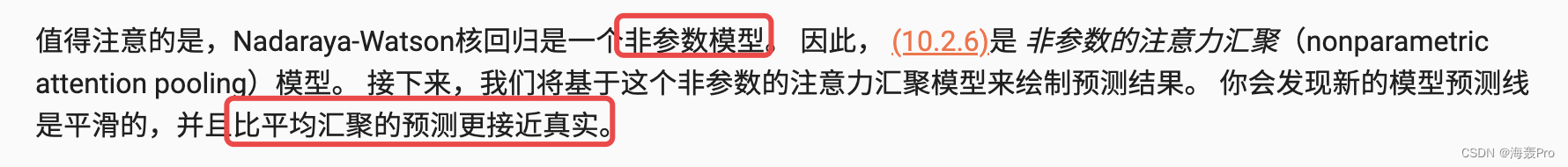
- 非参数模型:就是预测结果可用利用之前的数据直接计算出来,不需要额外的参数(学习参数)
X_repeat = x_test.repeat_interleave(n_train).reshape((-1, n_train))

attention_weights = nn.functional.softmax(-(X_repeat - x_train)**2 / 2, dim=1)

y_hat = torch.matmul(attention_weights, y_train)
plot_kernel_reg(y_hat)
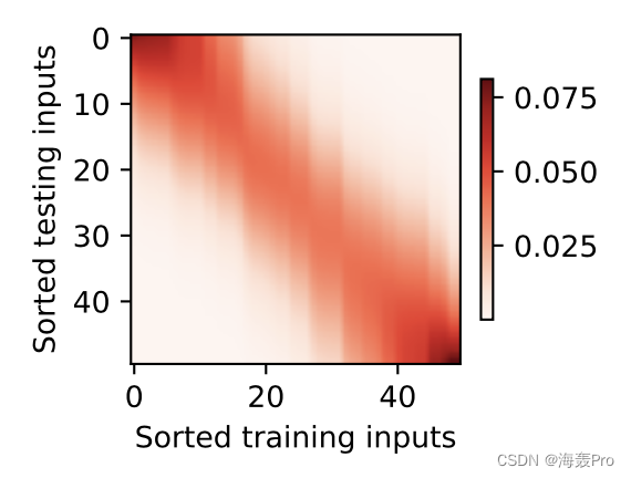
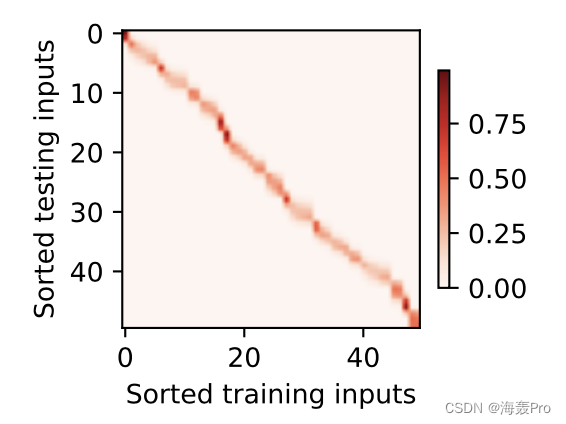
现在,我们来观察注意力的权重
这里 测试数据的输入相当于查询,而训练数据的输入相当于键
因为两个输入都是经过排序的,因此由观察可知”查询-键”对越接近, 注意力汇聚的注意力权重就越高
d2l.show_heatmaps(attention_weights.unsqueeze(0).unsqueeze(0),
                  xlabel='Sorted training inputs',
                  ylabel='Sorted testing inputs')
unsqueeze(0),在第0维插入一个维,默认为1
连续插入两次,得到(1,1,…) 也就是得到行数为1 列数为1(子图的数量,仅此而已)
参考:https://blog.csdn.net/ljwwjl/article/details/115342632
10.2.4. 带参数注意力汇聚

无参数时,完全由现有数据得到结果,需要大量的数据
可用添加一个可学习参数,这样可以通过一些数据进行训练,得到此参数
准确度会提高
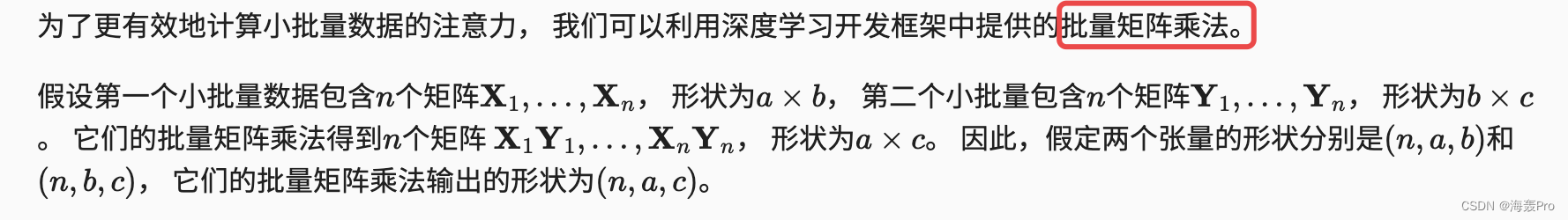
; 10.2.4.1. 批量矩阵乘法
X = torch.ones((2, 1, 4))
Y = torch.ones((2, 4, 6))
torch.bmm(X, Y).shape
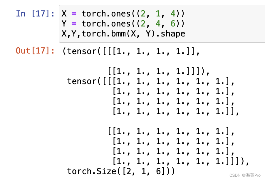
torch.bmm : 两个tensor的矩阵乘法
(2, 1, 6) = (2,1,4) * (2,4,6)
在注意力机制的背景中,我们可以使用小批量矩阵乘法来 计算小批量数据中的加权平均值。
weights = torch.ones((2, 10)) * 0.1
values = torch.arange(20.0).reshape((2, 10))
torch.bmm(weights.unsqueeze(1), values.unsqueeze(-1))
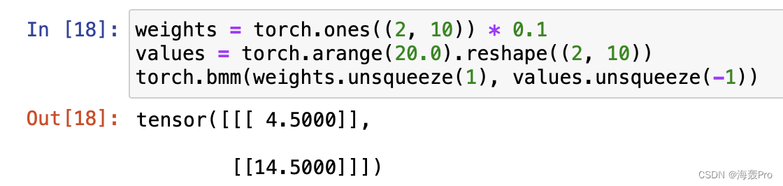
(2, 1, 1) = (2,1,10) * (2,10, 1)
10.2.4.2. 定义模型

class NWKernelRegression(nn.Module):
def __init__(self, **kwargs):
super().__init__(**kwargs)
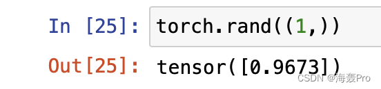
self.w = nn.Parameter(torch.rand((1,), requires_grad=True))
def forward(self, queries, keys, values):
queries = queries.repeat_interleave(keys.shape[1]).reshape((-1, keys.shape[1]))
self.attention_weights = nn.functional.softmax(
-((queries - keys) * self.w)**2 / 2, dim=1)
return torch.bmm(self.attention_weights.unsqueeze(1),
values.unsqueeze(-1)).reshape(-1)
Note
10.2.4.3. 训练

X_tile = x_train.repeat((n_train, 1))

Y_tile = y_train.repeat((n_train, 1))

keys = X_tile[(1 - torch.eye(n_train)).type(torch.bool)].reshape((n_train, -1))

values = Y_tile[(1 - torch.eye(n_train)).type(torch.bool)].reshape((n_train, -1))
训练带参数的注意力汇聚模型时,使用平方损失函数和随机梯度下降
net = NWKernelRegression()
loss = nn.MSELoss(reduction='none')
trainer = torch.optim.SGD(net.parameters(), lr=0.5)
animator = d2l.Animator(xlabel='epoch', ylabel='loss', xlim=[1, 5])

for epoch in range(5):
    trainer.zero_grad()
    l = loss(net(x_train, keys, values), y_train)
    l.sum().backward()
    trainer.step()
    print(f'epoch {epoch + 1}, loss {float(l.sum()):.6f}')
    animator.add(epoch + 1, float(l.sum()))
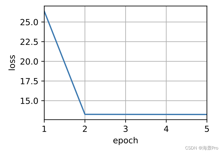
如下所示,训练完带参数的注意力汇聚模型后
我们发现: 在尝试拟合带噪声的训练数据时, 预测结果绘制的线不如之前非参数模型的平滑
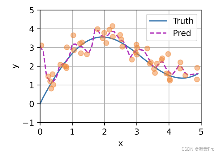
为什么新的模型更不平滑了呢?
我们看一下输出结果的绘制图:
- 与非参数的注意力汇聚模型相比,
- 带参数的模型加入可学习的参数后, *曲线在注意力权重较大的区域变得更不平滑
d2l.show_heatmaps(net.attention_weights.unsqueeze(0).unsqueeze(0),
                  xlabel='Sorted training inputs',
                  ylabel='Sorted testing inputs')
10.2.5. 小结
; 结语
学习资料: http://zh.d2l.ai/
文章仅作为个人学习笔记记录,记录从0到1的一个过程
希望对您有一点点帮助,如有错误欢迎小伙伴指正

Original: https://blog.csdn.net/weixin_44225182/article/details/126454693
Author: 海轰Pro
Title: 【Dive into Deep Learning / 动手学深度学习】第十章 – 第二节:注意力汇聚:Nadaraya-Watson 核回归
原创文章受到原创版权保护。转载请注明出处:https://www.johngo689.com/635454/
转载文章受原作者版权保护。转载请注明原作者出处!