使用JAGS训练贝叶斯回归模型

Fitting Baysian Regression Models Using JAGs

In Baysian statistics I use samples from the posterior distribution to answer inferential questions. The samples are generated by a Markov chain whose stationary distribution is the posterior. What this means is that not all samples generated by the Markov chain are from the posterior, but I usually have to let it run for some time before it reaches its stationary distribution.

Since I only want to use those samples for the analysis that were drawn from the posterior, it is crucial that I am able to assess whether the target distribution has been reached, that is, the Markov chain has converged.

When assessing concergence I will do a ‘visual inspection’ of the traceplot (is there good mixing between the chains?) and will look at the so-called scale-reduction factors of the parameters. This latter is called Gelman-Rubin diagnostic. The scale reduction factor quantifies the difference between the between-chain variance and whin-chain variance. If these are equal I get a scale-reduction factor of 1, while larger values mean that there is still a notable difference between chains. For both the visual inspection and the Gelman-Rubin diagnostic I will need multiple chains with differing starting points.

I will demonstrate convergence diagnostic with a Baysian linear regression problem.

Using density data

Union density is defined as the percentage of the work force who belongs to a trade union. There are a number of competing theories on what explains cross-national variation in union density.

To explore the different theories I use data from n = 20 n=20 n =2 0 countries with a continue histroy of democracy since World War II. I have the following variables:

• Union density (Uden);
• (log) Labour force size (LabF);
• Industrial concentration (IndC);
• Left wing givernment (LeftG);
  meansured id the late 1970s.

I fit the following (centred) linear regression model:
U d e n i ∼ N ( μ i , σ 2 ) Uden_i \sim N(\mu_i,\sigma^2)U d e n i ​∼N (μi ​,σ2 )
μ i = b 0 + b 1 ( L e f t G i − L e f t G ‾ ) + b 2 ( L a b F i − L a b F ‾ ) + b 3 ( I n d C i − I n d C ‾ ) \mu_i = b_0 + b_1(LeftG_i – \overline{LeftG}) + b_2(LabF_i – \overline{LabF}) + b_3(IndC_i – \overline{IndC})μi ​=b 0 ​+b 1 ​(L e f t G i ​−L e f t G ​)+b 2 ​(L a b F i ​−L a b F )+b 3 ​(I n d C i ​−I n d C )
with vague priors
1 / σ 2 ∼ G a m m a ( 0.001 , 0.001 ) b 0 ∼ N ( 0 , 1 0 5 ) b 1 ∼ N ( 0 , 1 0 5 ) b 2 ∼ N ( 0 , 1 0 5 ) b 3 ∼ N ( 0 , 1 0 5 ) 1/\sigma^2 \sim Gamma(0.001,0.001) \ b_0 \sim N(0,10^5) \ b_1 \sim N(0,10^5) \ b_2 \sim N(0,10^5) \ b_3 \sim N(0,10^5)1 /σ2 ∼G a m m a (0 .0 0 1 ,0 .0 0 1 )b 0 ​∼N (0 ,1 0 5 )b 1 ​∼N (0 ,1 0 5 )b 2 ​∼N (0 ,1 0 5 )b 3 ​∼N (0 ,1 0 5 )
I will fit the model, aeesee convergence, and discard any burn-in samples before making any posterior inference. For this I will run 2 separate chains and use Gelman_Rubin convergence disgnostic. Recall that when fitting a model previously I defined the jags model, coverted the data to a list, chose parameters of interest and specified starting values for all the chains. Now I will also consider burn-in periods, that is, choose the number of initial samples to be discard.

Firstly, I load the necessary packages:

{r library(R2jags) library(coda) library(lattice) library(MCMCvis) library(tidyverse)</p> <pre><code> To defin the model, I essentially translate the above model definition to the BUGS language line by line. Recall that in case of stochastic dependence I can't take advantage of the vertorised computation normally allowed by R, but I have to use a for loop. Also remember that JAGS uses the precision instead of the variance to parametrise the normal distribution. {r}
jags.model

I provide the data directly. Alternatively a cav file could be provide with colnumns Uden,LabF,LeftG and IndC. But here, since the data file is small, I omit having separate files. JAGS needs the data to be passed on as a list, thus I create a list from the defined data vectors, and call this list jags.data.

the data matrix
tmpdata

Next I set the parameters I want to monitor. At this stage these are the regression coefficients. I also specify initial values. TO check convergence I am planning to run 2 chains, thus I need two sets of initial values for the random parameters (ideally we should initialise all the stochastics nodes). These again should be passed on as a list. Note that Gelman-Rubbin convergence diagnostic is not possible with a single chain.

Parameters I want to monitor
jags.param

Sidenote: When defining initial values, I could specify the value of the variables separately, then add the variable names to the list (this is more convenient when the structure is more complex).

## Another way of creating the inits
tau= 100
b0= 40
b= c(10, -5, -25)
inits

Initial value can also be generated by random numbers, where the random number generators are added to a function

## Another way of creating the inits
jags.inits

The advantage of this latter method is that we can change the number of chains without having without having to worry about defining more or less initial values – sice jags will just call the above initial value function when in need of a new set of initial values. The disadvantage is that we have less control over the chosem initial values, and thatthis version can be harder to set up when the parameters, (including missing values) have a slighly more compler structure.

When fitting the model I set the number chains to tow (n.chains=2), draw 6000 samples for each chain (n.iter=6000), but discard the first 500 samples as burin-in (n.burnin=500). I also set n.thin to 1. This is because at this stage I want to keep all the samples. (Recall that he samples generated by the Markov chain are denendent samples. Ideally we would want indenpent, ot at least uncorrelated samples. To reduce correlation I could thin the generated samples, by taking only every nth sample, e.g. every 5th. This is what the thining argument does). Apart from the previously mentioned arguments, I also have to pass on the data, the list of initial values, the model definition and also the vector of parameters I wish to monitor.

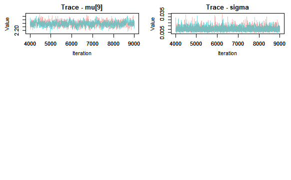
{r Fit the JAGS model jags.model.fit</p> <pre><code> To assess covergence I forst look at traceplots and check the mixing of the chains. Recall that there are multiple ways to generate traceplots. Here I use the **MCMCtrace** function of the **MCMCvis** package, which takes an MCMC object as it argument. The reason is that is the current version of **R2jags** there is a bug that, in certain cases, keeps some initak samples even when the burn-in values in high. These samples always show up when using **traceplot**, but with **MCMCvis** there is a better chance of seeing the true behaviour of the chains. **Q**: **Pruduce trace plots using the traceplot function and compare the results**. {r}
jagsfit.mcmc

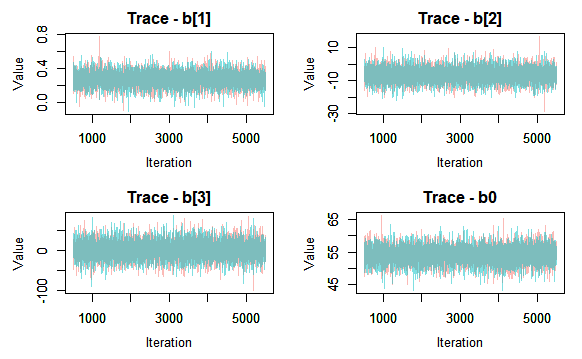
Here I see good mixing between the chains (heuristically this mean that the chains look like a random scatter around a stable value, and the behaviour of the two chains are indistinguishable).

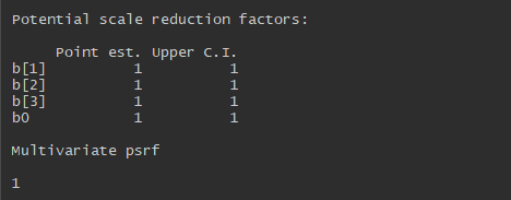
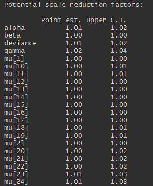
Traceplots on their own are not enough to access convergence, but they should be combined with Gelman-Rubin diagnostic. The gelman.diag() function can be used to extract the Gelman_Rubin test statistic values. Just as the MCMCtrace function nedds an MCMC object as its parameter.

gelman.diag(jagsfit.mcmc)

We can store these in a dataframe, which can be useful when I have a large number of parameters.

gelman.df

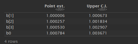
If the chains have converged, the Upper CI values should be close to 1 (anything above 1.1 usually indicates lack of convergence).

If the gelman.diag command doesn’t run I can try setting the multivariate argument to FALSE.

Here both the traceplots and the Gelman-Rubin values indicate convergence, but when there’s no convergence I can draw new samples using the update function:

jags.model.fit.upd

Q: Produce traceplots of the updated samples, is there still evidence of the bug?

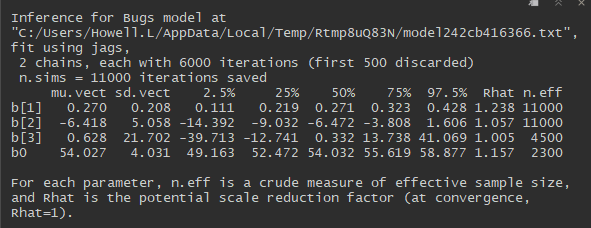
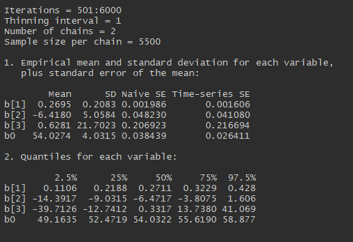
Once the convergence has been reached I can look at summary statistics and density plots of the posterior distribution. Note that Rhat column of the print output also provides estimates of the scale-reduction factor. However the gelman.diag() estimates with the upper cofidence interva;s are more reliable.

summary statistics
print(jags.model.fit)

If I use the summary function with the mcmc object, the MC standard error can also be assessed (this is given by the time-series SE column of the output). As a rule of thumb we want the MC error to be smaller than 1-5% of the posterior standard deviation (given in SD column).

summary(jagsfit.mcmc)

Q: Returen the model fitiing with a couple of different sample sizes and observe how the MC error changes in each case.

Note that the samples used in the above summary are all from the poserior distribution, since sonvergence has benn reached, and the initial 500 samples that we used as burn-in were discarded.

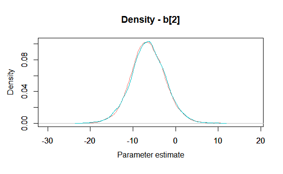
When looking at density plots the MCMCtrace function allows us to select specific parameter from a parameter vector. For example, we migh be interested in the coefficient of the labour force size(b 2 b_2 b 2 ​).

posterior density
MCMCtrace(
    jagsfit.mcmc,
    params = c('b\\[2\\]'),
    type = 'density',
    ind = TRUE,
    ISB = FALSE,
    exact = FALSE,
    pdf = FALSE
          )

Extracting the simulated samples allow me to make further inferences. As an example we will produce box plots of the posterior regression coefficients.

boxplot
beta

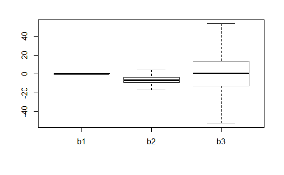
Data tend to favour Wallerstein’s theory (union density depends on labour force size), but I can’t draw strong conclusions from this analysis (notice that the 95% credible intervals for LabF and Indc both contain 0).

Exercise

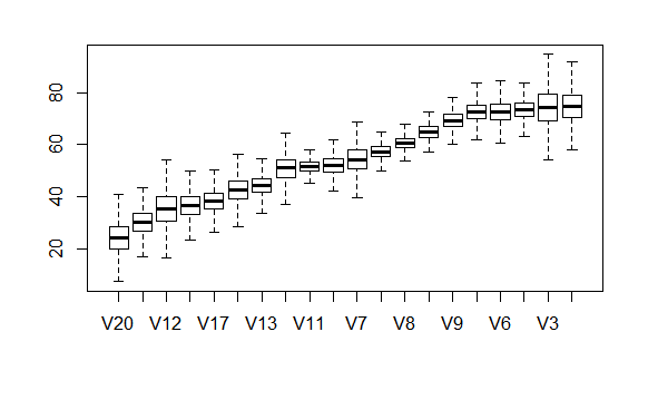
1. Produce a box plot of the posterior distribution of the mean union densities. Edit the plot to order the box plots by rank of the posterior mean union density. Hint: You will have to add mu to the list of monitored parameters and fit the model again. To create the boxplots, where the means are ordered according to their median rearrange the simulated samples for mu using mu[, order(apply(mu, 2, FUN=median))].

2. Edit the code to fit the same model, but with ‘uncentred’ covariates. How does this affect the convergence of the MCMC simulations and how does it affect the MC error?

3. Return the analysis first using the Wallerstein informative prior, then using the Stephens infrmative prior. Wallerstein and Stephens agree in the LeftG effect (and the vague intercept), but the two theories differ in their assumptions about the LabF effect and the IdcC effect.

4. Both Wallerstein and Stephens believe that left-waing governments assist union growth. Which translates a N ( 0.3 , 0.1 5 2 ) N(0.3,0.15^2)N (0 .3 ,0 .1 5 2 ) prior on the LeftG.

5. Wallerstein believes in negative labour force, and thus assumes a N ( − 5 , 2. 5 2 ) N(-5,2.5^2)N (−5 ,2 .5 2 ) prior on LabF effect, while keeps the vague N ( 0 , 1 0 5 ) N(0,10^5)N (0 ,1 0 5 ) prior for the Indc effect.

6. Stephens believes in postive industrial concentration effect, and thus assumes a N ( 10 , 5 2 ) N(10,5^2)N (1 0 ,5 2 ) prior for the IndC effect.

What conclusions can you draw?

## Solutions

1.

jags.param

2. Uncentred coviariates gives the following model definition:
jags.model

3. Model for Wallerstein informative prior:
jags.model.wallerstein

Dugongs

Baysian regression models can be easilly generalised to the non-linear case. To demonstrate this we will use the DUgong dataset. Furthermore I will also see how to make predictions and impute missing data.

Carlin and Gelfand (1991) consider data on length ( y i ) (y_i)(y i ​) and age ( x i ) (x_i)(x i ​) measurements for 27 dugongs (sea cows) captured off the Queensland.

To model the length of dugongs we can use a nonlinear growth vurve
y i ∼ N ( μ i , σ 2 ) μ i = α − β γ x i y_i \sim N(\mu_i,\sigma^2) \ \mu_i = \alpha – \beta\gamma^{x_i}y i ​∼N (μi ​,σ2 )μi ​=α−βγx i ​
where α , β > 0 γ ∈ ( 0 , 1 ) \alpha,\beta>0 \quad \gamma\in (0,1)α,β>0 γ∈(0 ,1 ).

Vague prior distributions with suitable constrains may be specified:
α ∼ U n i f ( 0 , 100 ) β ∼ U n i f ( 0 , 100 ) γ ∼ U n i f ( 0 , 1 ) \alpha \sim Unif(0,100) \ \beta \sim Unif(0, 100) \ \gamma \sim Unif(0,1)α∼U n i f (0 ,1 0 0 )β∼U n i f (0 ,1 0 0 )γ∼U n i f (0 ,1 )

Note that for α \alpha α and β \beta β I could also use a N ( 0 , 10000 ) N(0,10000)N (0 ,1 0 0 0 0 ) distribution restricted to the positive reals, that is dnorm(0, 0.00001);
T(0,) (note that T(,) is used for truncation where T(L,) means that the distribution is truncated below at value L T(,U) means it is truncated above at value U).

For the sampling variance, we could specify a uniform prior on log variance or log sd scale
l o g σ ∼ U n i f ( − 10 , 10 log\sigma \sim Unif(-10,10 l o g σ∼U n i f (−1 0 ,1 0
or gamma prior on precision scale.

Just as before, the dataset is small, so I will read it into R directlly.

age of dugongs
x

First we fit this model, check for convergence and look at posterior summary statistics.

To fit the model I just translate the above model definition line-by-line using the BUGS language.

jags.model

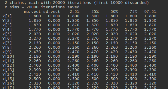
Next I set the paraeters I want to monitor, choose initial values for two chains, and fit the model, where I generate 10000 samples, and discard first 1000 as burn-in.

{r parameters I want to monitor jags.param</p> <pre><code> Next I check for convergence by producing traceplots and looking at the Gelman-Rubin statistic values. {r}
convert into MCMC object
jagsfit.mcmc

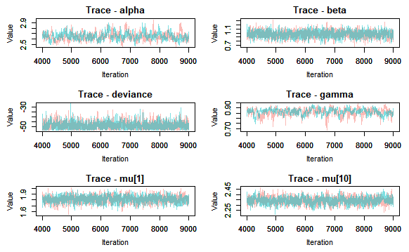
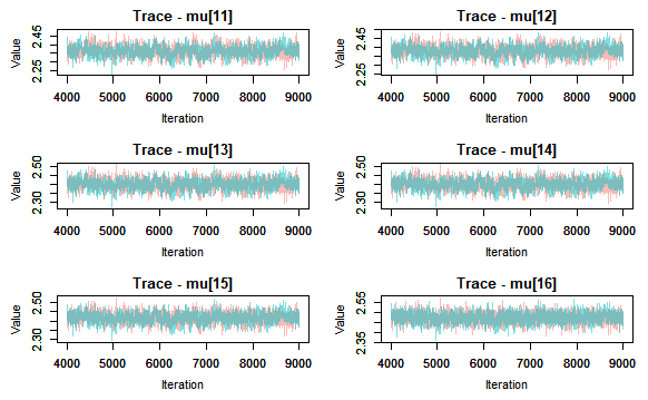
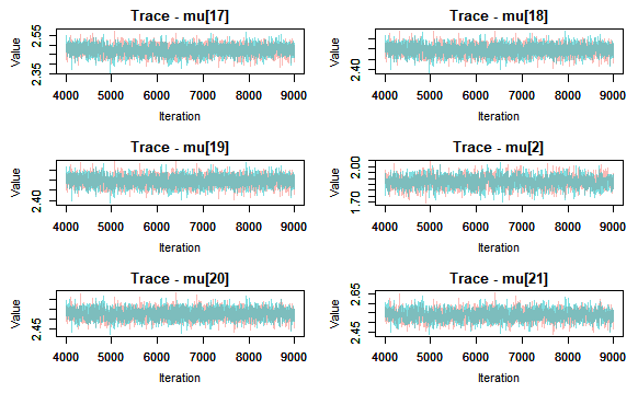
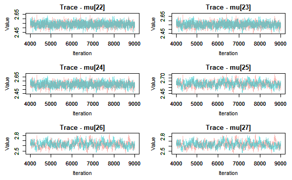
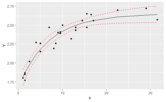
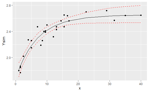
I can deduce that the model has converged, thus I can move onto looking at summary statistics, posterior density plots. And we can also plot the fitted model. This latter is done by extracting the mean and relevant percentiles of the posterior distribution, then using ggplot to plot these along with the meansurements. Here I will use rows of the summary statistics that correspond to the parameter mu.

summary statistics
print(jags.model.fit)

extract position of the mu parameters (check which rownames start with mu)
pos

Note that if I knew that the posterior was normal, I could have just used the mean and standard deviation of the posterior distribution to get the above plot. These can be extracted more esaily using the following code.

mu

As I can see fitting a non-linear model is just as straightforward in JAGS as a linear model. Even if there is no closed form solution available, it is still straightforward to obtain samples from posterior using MCMC.

I could explore the posterior further, but instead I now move onto discussing prediction.

It’s important to be able to predict unobserved quantiles for；

• ‘filling-in’ missing or censored data;

• model checking – are predictions ‘similar’ to oberved data?

• making predictions!

This is easy in JAGS; I just specify a stochastic node without a data-value – it will automatically predicted.

As an example, suppose we want to project beyond current observation in the dugong data, e.g. I might be interested at gugong length at ages 35 and 40.

There are two ways of doing, I can choose to set the prediction up as missing data, as mentioned before, and JAGS will automatically predict it. But I can also set up predictions explicity.

When making direct prediction we can add direct statements to our model definition to predict the gugong length at age 35 and 40. THat is, I get the following model definition.

jags.model

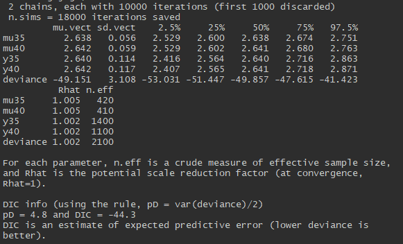
Note that the interval around mu40 will reflect uncertainty concerning fitted parameters. The interval around y40 will additionally reflectsampling error sigma and uncertainty about sigma.

Since now I have two extra stochastic nodes in the model definition, when specifing initial values I also have to account for these, and add initial values for y35 and y40 to the existing list.

inits1

Since I have already fitted the model without the prediction part, here I am only interested in the nodes I am predicting, so I set to monitor these variables. And finally fit the model.

{r Monitor the parameters I am using for the prediction jags.params</p> <pre><code> **Q**: _Check for convergence. Have all the nodes converged?_ Looking at summary statistics of the posterior of the monitored nodes gives us point and interval estimates for out predictions. _What are these?_ {r}
get point and interval estimates
print(jags.model.fit)

Next I move onto the second prediction method.

I can set up prediction as missing data, and JAGS will automatically predict it. In this case I use the original model definition, but a modeified dataset. Generally, imputing missing data as a method of prediction is easier, but I do have to do a lit more work when initialsing the chains.

In the modified dataset I treat the observations corresponding to
x=35, and x=40 as missing

x

Recall that all unknown quantities (including missing data!) should still be initialised. Since the ‘missing values’ are part of the data that I pass onto JAGS, I need to use this data structure when initialising the chains. That is, we use NA where the data in available (since these are not stochastic nodes), and initialise where data is missing. In the model deginition, where the data is missing, Y[i]~dnorm(mu[i],tau) is essentially a prior on these missing values.

{r inits1</p> <pre><code> Now I am ready to fit the model. {r
Fit JAGS
jags.model.fit

When looking at the outcome (you should also check for convergence) I extract point and interval estimates and also plot to fitted model. Note that the first 27 Y nodes are not stochastic, since I have data available there. But since I am monitoring these too, they will appear in the output of the print function.

print model fit
print(jags.model.fit)

extract position of the mu parameters (check with rownames start with mu)
pos

Notice how in the above plot the two missing values got imputed. However we have greater uncertainty around these nodes.

Exercise

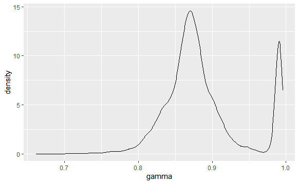
1. Change the prior in the original model (without prediction) to being uniform on l o g ( σ ) log(\sigma)l o g (σ): is there any influence? (Note – you must always specify initial values for the stochastic parameters, i.e. the parameters assigned prior distribution, so you will need to edit the initial values files here as well as the model code.) Also remember that you cannot specify a function of parameters on the left side of a distribution in the BUGS language, so you will need to create a new variable equal to l o g ( σ ) log(\sigma)l o g (σ) and assign this new variable an appropriate prior. Since BUGS does not allow the same variable to appear more than once on the left side of a statement, you will need to specify this new variable using the following format:
   function.of.sigma<- new.variable< code><br>rather than<br><code>new.variable<- function.of.sigma< code><br>Check the posterior distribution for <span class="katex--inline"><span class="katex"><span class="katex-mathml">&#x3B3; \gamma</span><span class="katex-html"><span class="base"><span class="mord mathdefault">&#x3B3;</span></span></span></span></span>: do you think the uniform prior on this parameter is very influential?<!-----></code><!----->

jags.model

1. Use both method to obtain prediction at age 25 and 33. How do these look compared to the predictions aat age 35 and 40?

2. We can also use prediction as model checking. Edit the model definition so that it includes a statement to calculate the predictive for each Y.pred[i]

Here I work with the original dataset again
But I add an extra variable to the for loop of the model definition

x

Original: https://blog.csdn.net/o_hoooo/article/details/119891919
Author: 「已注销」
Title: 使用JAGS训练贝叶斯回归模型