NumPy Application: Determining Moore‘s Law with real data in NumPy

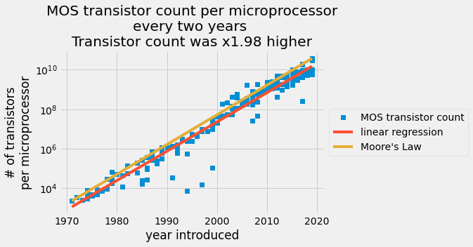
每个给定芯片上的晶体管数量绘制在 y 轴上的对数刻度上，线性刻度上的引入日期在 x 轴上。
蓝色的点表示晶体管记数表；红色的线是最小二乘预测；橙色的线是摩尔定律
将要做的事
背景知识：1965年，工程师Gordon Moore预测在未来十年内，芯片上的晶体管数量将每两年翻一番。
本篇将在摩尔预测之后的53年将其预测与实际晶体管数量进行比较。
与摩尔定律相比，将确定最适合的常数来描述半导体上晶体管的指数增长。
本篇涉及到的知识

• 从*.csv文件中加载数据
• 使用最小二乘法来执行线性回归并预测指数增长
• 比较模型之间的指数增长常数
• 将分析结果存储为.npz和.csv文件中
• 评估半导体制造商在过去五年中取得的进步

接下来会使用到的函数功能说明

• np.loadtxt:this function loads text into a Numpy array
• np.log:this function takes the natural log(自然对数) of all elements in a Numpy array
• no.exp:this function takes the exponential of all elements in a Numpy array（计算以e为底的指数）
• lamba:this is a minimal function definition for creating a function model(创建模型的最小函数定义)
• plt.semilogy:this function will plot x-y data onto a figure with a linear x-axis and log10 y-axis（此函数会将 x-y 数据绘制到具有线性 x 轴和 log10 y 轴的图形上）
• plt.plot:this function will plot x-y data on linear axes;
• sm.OLS :find fitting parameters and standard errors using the statsmodels ordinary least squares model(使用 statsmodels 普通最小二乘模型查找拟合参数和标准误差)
• slicing arrays:view parts of the data loaded into the workspace,slice the arrays.e.g.x[:10] for the first 10 values in the array,x
• boolean array indexing:to view parts of the data that match a given condition use boolean operations to index an array
• np.block:to combine arrays into 2D arrays
• np.newaxis:to change a 1D vector to a row or column vector
• np.savaz an np.savatxt:these two functions will save your arrays in zipped array format and txt,respectively

moore law
1.您的经验模型假设每个半导体的晶体管数量呈指数增长，ln(transistor_count) = f(year) = A * year + B, A,B是fitting constant；式子变形得 transisor_count = e(Am*year+Bm)(Am,Bm,是每两年晶体管数量翻一番的常数，从 1971 年的 2250 个晶体管开始)

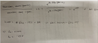
算出Am = 0.3466，Bm = -675.4

A_M = np.log(2) / 2
B_M = np.log(2250) - A_m * 1971
Moores_law = lambda year: np.exp(B_M) * np.exp(A_M * year)

ML_1971 = Moores_law(1971)
ML_1973 = Moores_law(1973)
print("In 1973,G. moore {:.0f} transistors on Intels chip".format(ML_1971))
print("This is x{:.2f} more transistors than 1971".format(ML_1973 / ML_1971))

> In 1973, G. Moore expects 4500 transistors on Intels chips This is
> x2.00 more transistors than 1971

将历史工厂的数据加载到工作区间

NOW，make a prediction based upon the historical data for semiconductors per chip.

! head transistor_data.csv
'''
Processor,MOS transistor count,Date of Introduction,Designer,MOSprocess,Area
Intel 4004 (4-bit  16-pin),2250,1971,Intel,"10,000 nm",12 mm²
Intel 8008 (8-bit  18-pin),3500,1972,Intel,"10,000 nm",14 mm²
NEC μCOM-4 (4-bit  42-pin),2500,1973,NEC,"7,500 nm",?

Intel 4040 (4-bit  16-pin),3000,1974,Intel,"10,000 nm",12 mm²
Motorola 6800 (8-bit  40-pin),4100,1974,Motorola,"6,000 nm",16 mm²
Intel 8080 (8-bit  40-pin),6000,1974,Intel,"6,000 nm",20 mm²
TMS 1000 (4-bit  28-pin),8000,1974,Texas Instruments,"8,000 nm",11 mm²
MOS Technology 6502 (8-bit  40-pin),4528,1975,MOS Technology,"8,000 nm",21 mm²
Intersil IM6100 (12-bit  40-pin; clone of PDP-8),4000,1975,Intersil,,
'''

data = np.loadtxt("transistor_data.csv",delimiter=",",usecols=[1,2],skiprows=1)

year = data[:,1]
transistor_count=data[:,0]
print("year:\t\t",year[:10])
print("trans. cnt.:\t\t",transistor_count[:10])

现在创建一个预测函数来预测特定年份的transistor count

yi=np.log(transistor_count)

计算历史数据的增长曲线

在上面已经将transistor_count 作为因变量，yi年份作为自变量，其中自变量转换为对数指数函数
yi = A _year + B.
现在寻找一个best-fit model来最小化yi和A_year+B之间的差距,使用最小二乘法

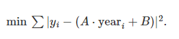
这里的y是晶体管的数据，1D array,
Z=[year1,year2]

Z=year[:, np.newaxis] ** [1, 0]
model=sm.OLS(yi,Z)

results=model.fit()
print(results.summary())

AB = results.params
A = AB[0]
B = AB[1]
transistor_count_predicted = np.exp(B) * np.exp(A * year)
transistor_Moores_law = Moores_law(year)
plt.style.use("fivethirtyeight")
plt.semilogy(year, transistor_count, "s", label="MOS transistor count")
plt.semilogy(year, transistor_count_predicted, label="linear regression")

plt.plot(year, transistor_Moores_law, label="Moore's Law")
plt.title(
    "MOS transistor count per microprocessor\n"
    + "every two years \n"
    + "Transistor count was x{:.2f} higher".format(np.exp(A * 2))
)
plt.xlabel("year introduced")
plt.legend(loc="center left", bbox_to_anchor=(1, 0.5))
plt.ylabel("# of transistors\nper microprocessor")

将结果另存为其他格式分享

The last step,is to share your findings.

1.np.savez:save Numpy arrays for other Python sessions
2.np.savetxt:save a csv file with the original data and your predicted data
zipping the arrays into a file
np.savez 将数以千计的数据保存起来并赋一个名字
np.load 可以将保存的数据重新加载回来
下面将保存 year,transistor count,predicted transistor count,Gordon Moore’s predicted count,and fitting constants.

再另加一个notes变量，使得读者可以理解文件的内容

notes = "the arrays in this file are the result of a linear regression model\n"
notes += "the arrays include\nyear: year of manufacture\n"
notes += "transistor_count: number of transistors reported by manufacturers in a given year\n"
notes += "transistor_count_predicted: linear regression model = exp({:.2f})*exp({:.2f}*year)\n".format(
    B, A
)
notes += "transistor_Moores_law: Moores law =exp({:.2f})*exp({:.2f}*year)\n".format(
    B_M, A_M
)
notes += "regression_csts: linear regression constants A and B for log(transistor_count)=A*year+B"
print(notes)
'''
the arrays in this file are the result of a linear regression model
the arrays include
year: year of manufacture
transistor_count: number of transistors reported by manufacturers in a given year
transistor_count_predicted: linear regression model = exp(-666.33)*exp(0.34*year)
transistor_Moores_law: Moores law =exp(-675.38)*exp(0.35*year)
regression_csts: linear regression constants A and B for log(transistor_count)=A*year+B
'''
np.savez(
    "mooreslaw_regression.npz",
    notes=notes,
    year=year,
    transistor_count=transistor_count,
    transistor_count_predicted=transistor_count_predicted,
    transistor_Moores_law=transistor_Moores_law,
    regression_csts=AB,
)
results = np.load("mooreslaw_regression.npz")
print(results["regression_csts"][1])

！ ls
'''
mooreslaw_regression.csv
mooreslaw_regression.npz
mooreslaw-tutorial.md
pairing.md
save-load-arrays.md
_static
text_preprocessing.py
transistor_data.csv
tutorial-deep-learning-on-mnist.md
tutorial-deep-reinforcement-learning-with-pong-from-pixels.md
tutorial-ma.md
tutorial-nlp-from-scratch
tutorial-nlp-from-scratch.md
tutorial-plotting-fractals
tutorial-plotting-fractals.md
tutorial-static_equilibrium.md
tutorial-style-guide.md
tutorial-svd.md
tutorial-x-ray-image-processing
tutorial-x-ray-image-processing.md
who_covid_19_sit_rep_time_series.csv
x_y-squared.csv
x_y-squared.npz
'''

np.savez 的好处是你可以保存数百个不同形状和类型的数组

创建自己的csv（comma separated value）文件

如果要共享数据并在表格中查看结果，则必须创建一个文本文件。使用 np.savetxt 保存数据。这个功能比 np.savez 更受限制。分隔文件，如 csv 文件，需要二维数组。

通过创建一个新的二维数组来准备要导出的数据，该数组的列包含要保存的数据。

使用标题选项来描述数据和文件的列。定义另一个包含文件信息的变量作为头。

head = "the columns in this file are the result of a linear regression model\n"
head += "the columns include\nyear: year of manufacture\n"
head += "transistor_count: number of transistors reported by manufacturers in a given year\n"
head += "transistor_count_predicted: linear regression model = exp({:.2f})*exp({:.2f}*year)\n".format(
    B, A
)
head += "transistor_Moores_law: Moores law =exp({:.2f})*exp({:.2f}*year)\n".format(
    B_M, A_M
)
head += "year:, transistor_count:, transistor_count_predicted:, transistor_Moores_law:"
print(head)

由于csv文件是个表格，但表格数据本是就是2D的。
首先创建一个2D array用来导出至csv。
使用 year, transistor_count, transistor_count_predicted, and transistor_Moores_law 分别当作第一列到第四列
将计算常量放在header，因为他们的shape不是（179，）
np.block 函数将数组附加在一起以创建一个新的更大的数组。
使用np.newaxis将1D 向量转变成 columns(列) 即（179，）–> (179, 1)这样可以用于matrix computing

>>> year.shape

>>> year[:,np.newaxis].shape

output = np.block(
    [
        year[:, np.newaxis],
        transistor_count[:, np.newaxis],
        transistor_count_predicted[:, np.newaxis],
        transistor_Moores_law[:, np.newaxis],
    ]
)
np.savetxt("mooreslaw_regression.csv",X=output,delimiter=",",header=head)
! head mooreslaw_regression.csv
'''
the columns in this file are the result of a linear regression model
the columns include
year: year of manufacture
transistor_count: number of transistors reported by manufacturers in a given year
transistor_count_predicted: linear regression model = exp(-666.33)*exp(0.34*year)
transistor_Moores_law: Moores law =exp(-675.38)*exp(0.35*year)
year:, transistor_count:, transistor_count_predicted:, transistor_Moores_law:
1.971000000000000000e+03,2.250000000000000000e+03,1.130514785642334573e+03,2.249999999999916326e+03
1.972000000000000000e+03,3.500000000000000000e+03,1.590908400344209895e+03,3.181980515339620069e+03
1.973000000000000000e+03,2.500000000000000000e+03,2.238793840142230238e+03,4.500000000000097316e+03
'''

参考网站：
https://numpy.org/numpy-tutorials/content/mooreslaw-tutorial.html

Original: https://blog.csdn.net/qiugengjun/article/details/122192872
Author: 看到就想笑
Title: NumPy Application: Determining Moore‘s Law with real data in NumPy