第五课：回归分析

目录

一 线性回归

1.理论​

2.代码

二 非线性回归

1.理论

三 Nonparametric methods

3.1理论

3.2Decision Trees

3.3代码

四 APP使用

一 线性回归

2.代码

% Perform the parametric linear regression
clear, close all
clc

%% load Advertising data:
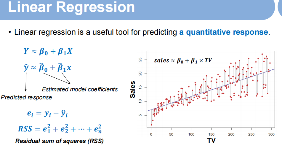
% Sales (in thousands of units) for a particular product as a function of advertising budgets
% (in thousands of dollars) for TV, radio, and newspaper media.

[num,txt,raw]=xlsread('Advertising.csv');
Sales=num(:,5);
TV=num(:,2);
Radio=num(:,3);
Newspaper=num(:,4);

%% Perform univariate linear regression on TV advertising budget
%%% Regress "Sales" on "TV"
mdl_tv = fitlm(TV,Sales)
% mdl_tv.Coefficients
% mdl_tv.RMSE
% mdl_tv.Rsquared.Ordinary

figure,
scatter(TV,Sales), hold on
plot([min(TV), max(TV)],[predict(mdl_tv,min(TV)), predict(mdl_tv,max(TV))],'k-','linewidth',2)
xlabel('TV budgets'), ylabel('Sales of product')
title(['Sales=' num2str(mdl_tv.Coefficients.Estimate(1)) '+' ...

          num2str(mdl_tv.Coefficients.Estimate(2)) '*TV',...

          ', R^2=' num2str(mdl_tv.Rsquared.Ordinary)])

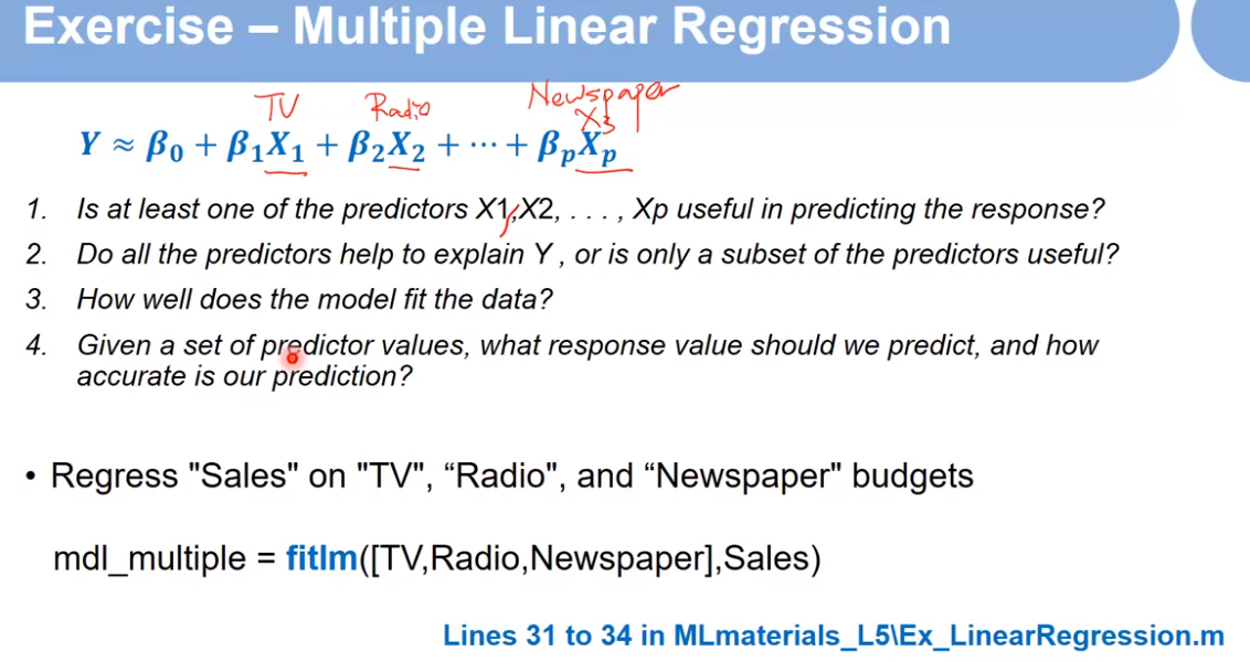
%% Perform multiple linear regression on all advertising budgets
mdl_multiple = fitlm([TV,Radio,Newspaper],Sales)

%%% check the correlations between different types of budgets
[rho,p]=corr([TV,Radio,Newspaper]);

结果如下：

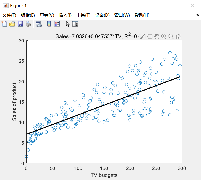
scatter(TV,Sales) 画出散点图

mdl_tv = fitlm(TV,Sales) 表示单因子线性回归分析

plot([min(TV), max(TV)],[predict(mdl_tv,min(TV)), predict(mdl_tv,max(TV))],’k-‘,’linewidth’,2)

[min(TV), max(TV)] 给出图形的范围

predict函数表示给定一个模型，还有一个输入参数，能够得出模型的输出参数

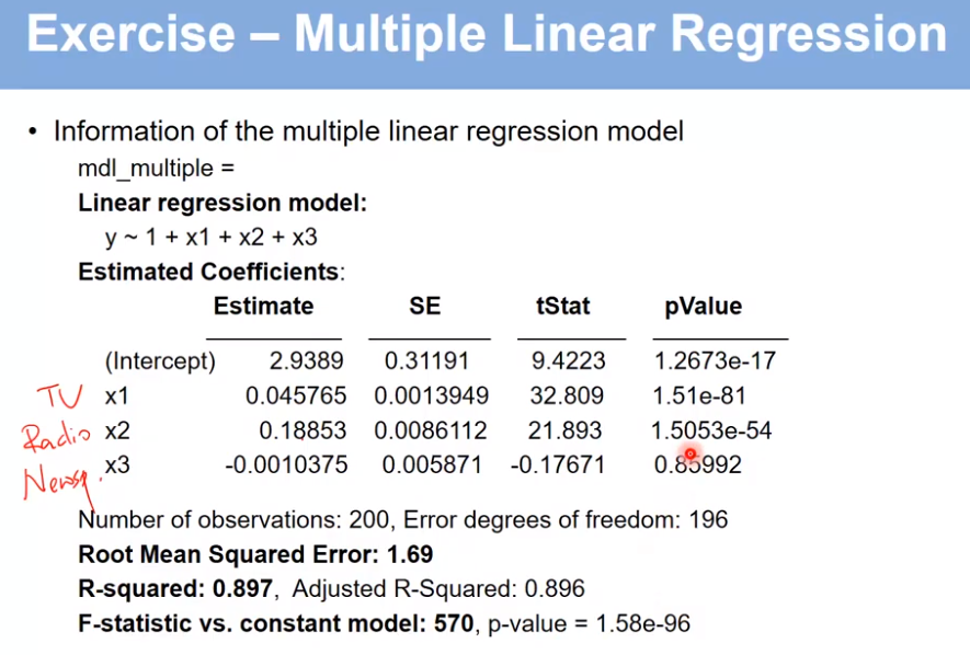
mdl_multiple = fitlm([TV,Radio,Newspaper],Sales) 多因子回归分析

[rho,p]=corr([TV,Radio,Newspaper]) 衡量三个系数之间的相关性。

rho得出任意两个系数之间的相关系数，是一个系数矩阵，越大则相关性越强；p得出相关系数的显著性，是一个矩阵，越小则越显著

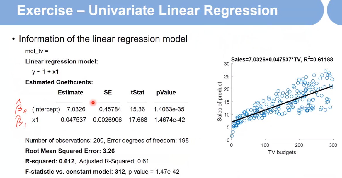
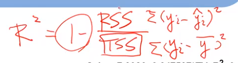
R^2：代表拟合效果，越接近1越好。 F：越大越好 pValue：代表显著性，越小越好

二 非线性回归

1.理论

% Perform the parametric polynomial regression
clear, close all

%% load Auto data:
[num,txt,raw]=xlsread('Auto.csv');
mpg=num(:,1); % gas mileage in miles per gallon
horsepower=num(:,4);

excludeind=find(isnan(horsepower));  % identify the indices with missing horsepower data
mpg(excludeind,:)=[]; % remove the observations with missing horsepower data
horsepower(excludeind,:)=[]; % remove the observations with missing horsepower data

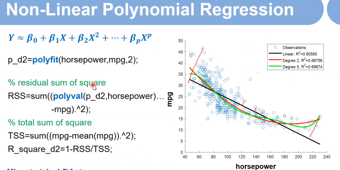
%% perform polynomial regression
p_d1=polyfit(horsepower,mpg,1); % linear
RSS=sum((polyval(p_d1,horsepower)-mpg).^2); % residual sum of square
TSS=sum((mpg-mean(mpg)).^2); % total sum of square
R_square_d1=1-RSS/TSS;

p_d2=polyfit(horsepower,mpg,2); % Degree 2
RSS=sum((polyval(p_d2,horsepower)-mpg).^2); % residual sum of square
TSS=sum((mpg-mean(mpg)).^2); % total sum of square
R_square_d2=1-RSS/TSS;

p_d5=polyfit(horsepower,mpg,5); % Degree 5
RSS=sum((polyval(p_d5,horsepower)-mpg).^2); % residual sum of square
TSS=sum((mpg-mean(mpg)).^2); % total sum of square
R_square_d5=1-RSS/TSS;

figure,
scatter(horsepower,mpg), hold on
x=sort(horsepower);
plot(x,polyval(p_d1,x),'k-','linewidth',2)
plot(x,polyval(p_d2,x),'r-','linewidth',2)
plot(x,polyval(p_d5,x),'g-','linewidth',2)
xlabel('horsepower'), ylabel('mpg')
legend('Observations',...

             ['Linear, R^2=' num2str(R_square_d1)],...

             ['Degree 2, R^2=' num2str(R_square_d2)],...

             ['Degree 5, R^2=' num2str(R_square_d5)])

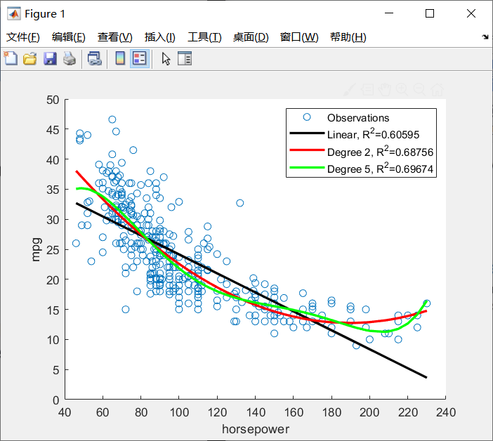
p_d2=polyfit(horsepower,mpg,2);

horsepower：输入，x轴 mpg：y轴 2：最高只有2次项

polyval(p_d2,horsepower) 预测函数

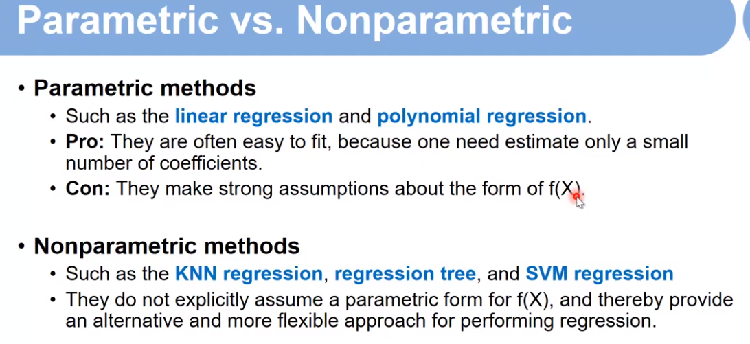
三 Nonparametric methods

3.1理论

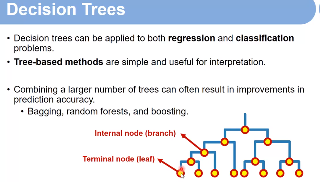
3.2Decision Trees

3.3代码

准备数据集，数据预处理

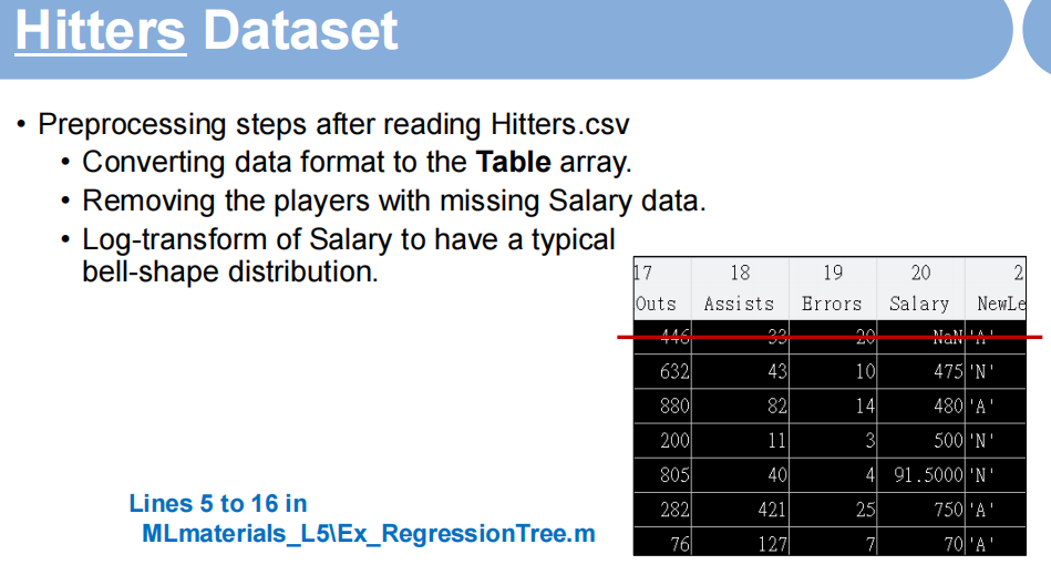
将数据转换为table类型，并且第一行的数据不转换：

data=cell2table(raw(2:end,:))       

定义变量名：

for i=1:size(data,2)
    data.Properties.VariableNames{i}=raw{1,i}; % assign the VariableNames
end

去除无用数据：

excludeind=find(isnan(data.Salary));  % identify the indices with missing Salary data
data(excludeind,:)=[]; % remove the players with missing Salary data

取log函数（其实是ln，自然对数为底）使数据更平滑：

data.Salary=log(data.Salary); % log-transform to have a typical bell-shape distribution

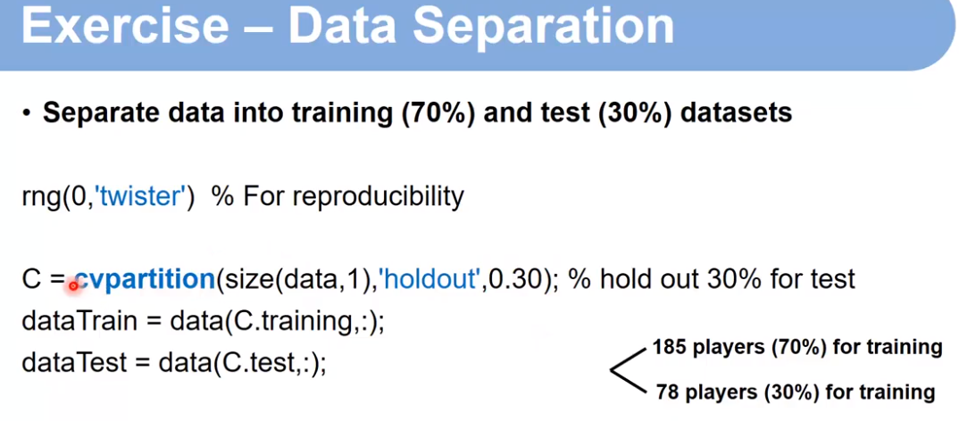
数据集分解：

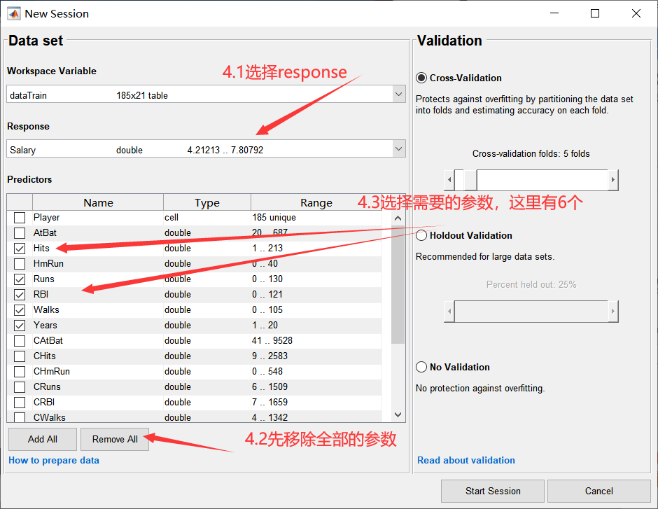
建立模型

第一步：

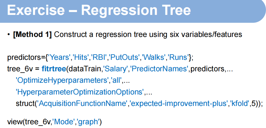
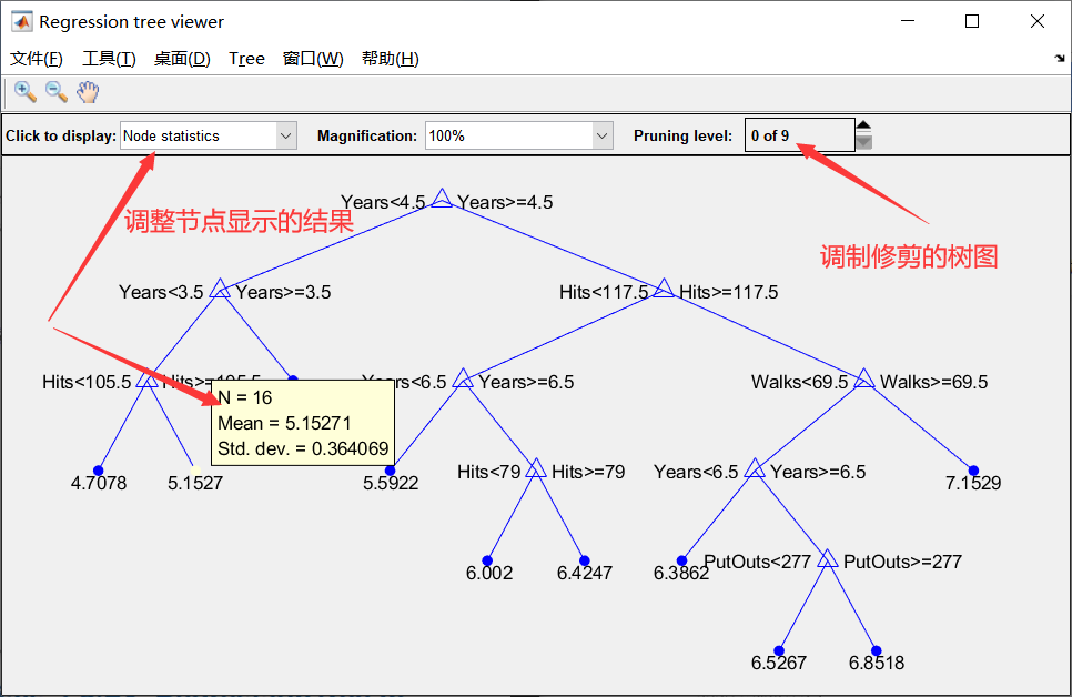
选定六个指标；选定salary作为衡量标准，交叉验证，分为5折；view函数为画出树图，如下：

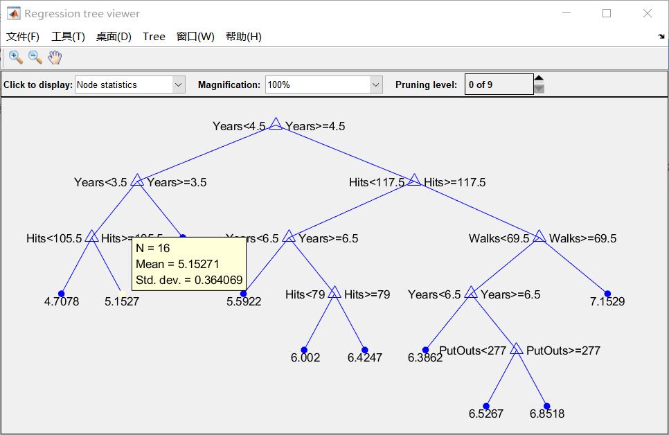
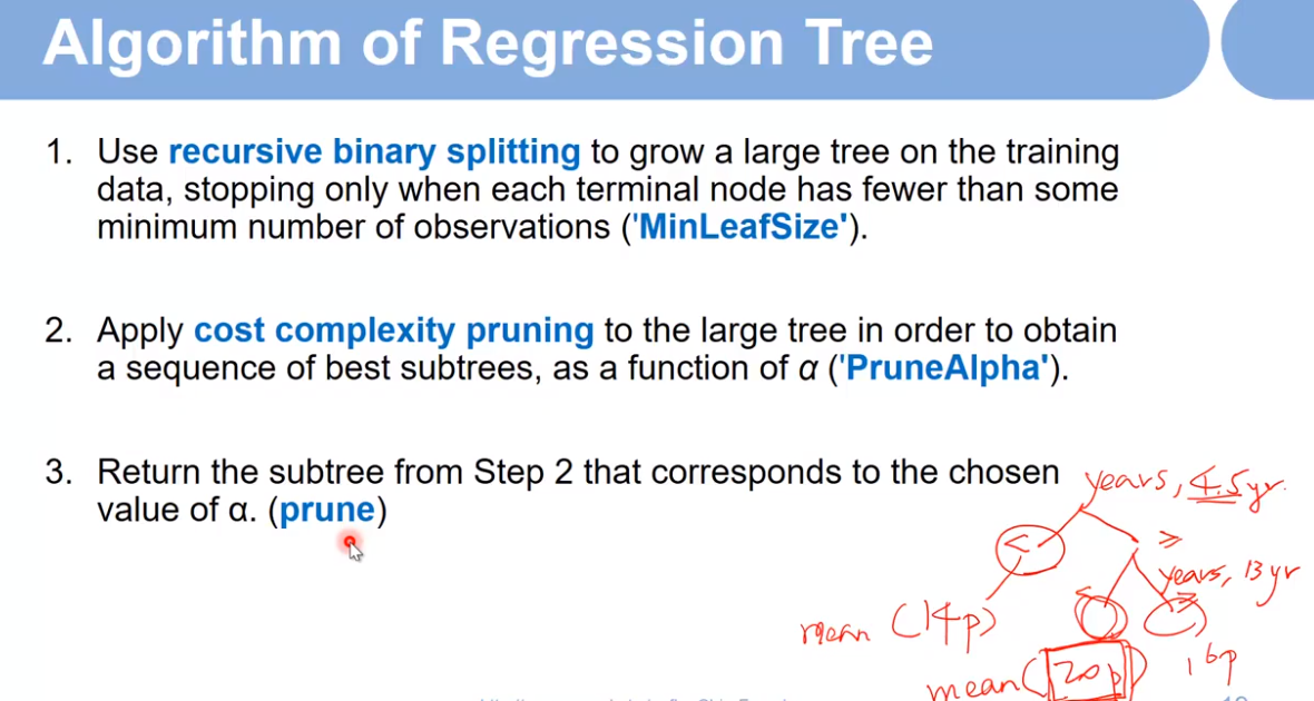
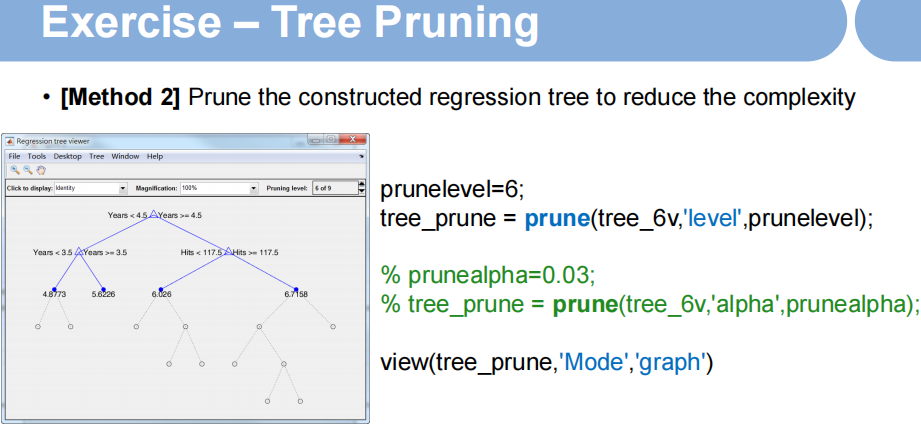
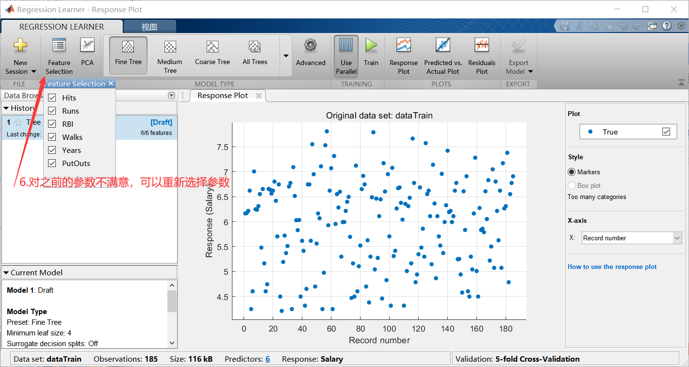
第二步：修建树图

改prunelevel或者prunealpha

也可以直接在图片上面修改：

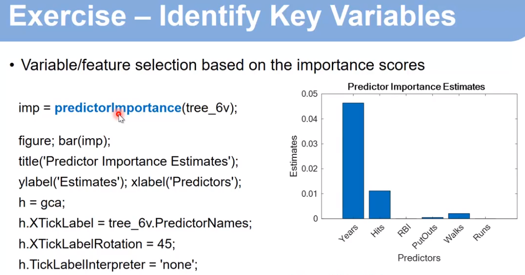
查看参数的重要程度：

imp = predictorImportance(tree_6v);

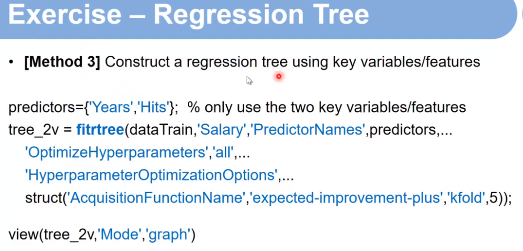
第三步：只用两个参数运行模型

完整代码：

% Perform the regression tree using "fitrtree" function
clear, close all

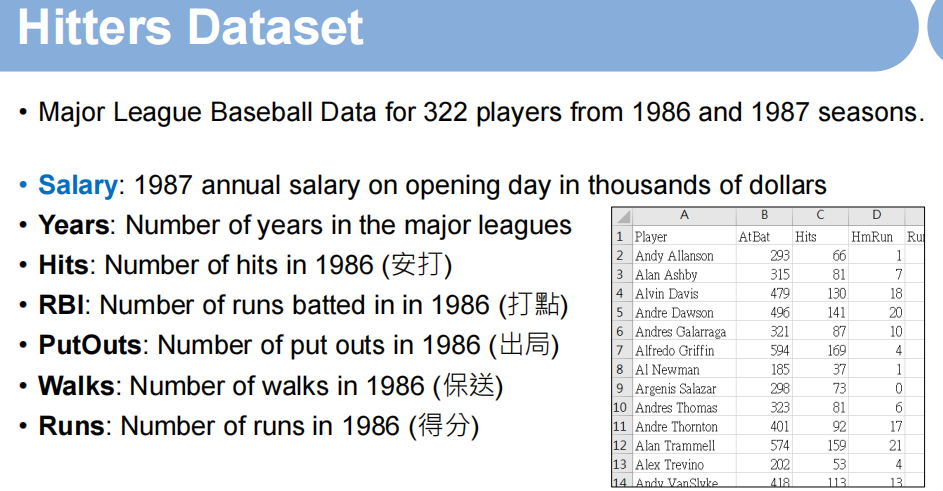
%% load Hitters data: Major League Baseball Data from the 1986 and 1987 seasons.

[num,txt,raw]=xlsread('Hitters.csv');

% construct Table array
data=cell2table(raw(2:end,:));
for i=1:size(data,2)
    data.Properties.VariableNames{i}=raw{1,i}; % assign the VariableNames
end
excludeind=find(isnan(data.Salary));  % identify the indices with missing Salary data
data(excludeind,:)=[]; % remove the players with missing Salary data

data.Salary=log(data.Salary); % log-transform to have a typical bell-shape distribution

%% Separate data into training (70%) and test (30%) datasets
rng(0,'twister')  % For reproducibility，可删除这一行代码，只是为了保证随机数是一样的

C = cvpartition(size(data,1),'holdout',0.30); % randomly hold out 30% of subjects for test
dataTrain = data(C.training,:);
dataTest = data(C.test,:);

%% [Method 1] Construct a regression tree using six variables/features
% Construct a regression tree using the training dataset
predictors={'Years','Hits','RBI','PutOuts','Walks','Runs'};
tree_6v = fitrtree(dataTrain,'Salary','PredictorNames',predictors,...

    'OptimizeHyperparameters','all',...

    'HyperparameterOptimizationOptions',...

    struct('AcquisitionFunctionName','expected-improvement-plus','kfold',5));
view(tree_6v,'Mode','graph')

% Test the tree model on the test dataset
Salary_predict=predict(tree_6v,dataTest);
MSE=loss(tree_6v,dataTest);  % mean squared error, MSE=mean((Salary_predict-dataTest.Salary).^2);

RSS=sum((Salary_predict-dataTest.Salary).^2); % residual sum of square
TSS=sum((dataTest.Salary-mean(dataTest.Salary)).^2); % total sum of square
R_square=1-RSS/TSS;

figure,plot(1:size(dataTest,1),dataTest.Salary,'r.-',1:1:size(dataTest,1),Salary_predict,'b.-')
title(['[Method 1] MSE = ' num2str(MSE) ', R^2 = ' num2str(R_square)])
legend('True salaries','Predicted salaries')
xlabel('Players'),ylabel('Salaries')

%% [Method 2] Construct a regression tree using six variables/features with pruning
prunelevel=6;
tree_prune = prune(tree_6v,'level',prunelevel);

% prunealpha=0.03;
% tree_prune = prune(tree_6v,'alpha',prunealpha);

view(tree_prune,'Mode','graph')

% Test the tree model on the test dataset
Salary_predict=predict(tree_prune,dataTest);
MSE=loss(tree_prune,dataTest);  % mean squared error, MSE=mean((Salary_predict-dataTest.Salary).^2);

RSS=sum((Salary_predict-dataTest.Salary).^2); % residual sum of square
TSS=sum((dataTest.Salary-mean(dataTest.Salary)).^2); % total sum of square
R_square=1-RSS/TSS;

figure,plot(1:size(dataTest,1),dataTest.Salary,'r.-',1:1:size(dataTest,1),Salary_predict,'b.-')
title(['[Method 2] MSE = ' num2str(MSE) ', R^2 = ' num2str(R_square)])
legend('True salaries','Predicted salaries')
xlabel('Players'),ylabel('Salaries')

%% Variable/Feature selection based on the importance scores
imp = predictorImportance(tree_6v);

figure;
bar(imp);
title('Predictor Importance Estimates');
ylabel('Estimates');
xlabel('Predictors');
h = gca;
h.XTickLabel = tree_6v.PredictorNames;
h.XTickLabelRotation = 45;
h.TickLabelInterpreter = 'none';

%% [Method 3] Construct a regression tree using key variables/features
% Construct a regression tree using the training dataset
predictors={'Years','Hits'};  % only use the two key variables/features
tree_2v = fitrtree(dataTrain,'Salary','PredictorNames',predictors,...

    'OptimizeHyperparameters','all',...

    'HyperparameterOptimizationOptions',...

    struct('AcquisitionFunctionName','expected-improvement-plus','kfold',5));
view(tree_2v,'Mode','graph')

% Test the tree model on the test dataset
Salary_predict=predict(tree_2v,dataTest);
MSE=loss(tree_2v,dataTest);  % mean squared error, MSE=mean((Salary_predict-dataTest.Salary).^2);

RSS=sum((Salary_predict-dataTest.Salary).^2); % residual sum of square
TSS=sum((dataTest.Salary-mean(dataTest.Salary)).^2); % total sum of square
R_square=1-RSS/TSS;

figure,plot(1:size(dataTest,1),dataTest.Salary,'r.-',1:1:size(dataTest,1),Salary_predict,'b.-')
title(['[Method 3] MSE = ' num2str(MSE) ', R^2 = ' num2str(R_square)])
legend('True salaries','Predicted salaries')
xlabel('Players'),ylabel('Salaries')

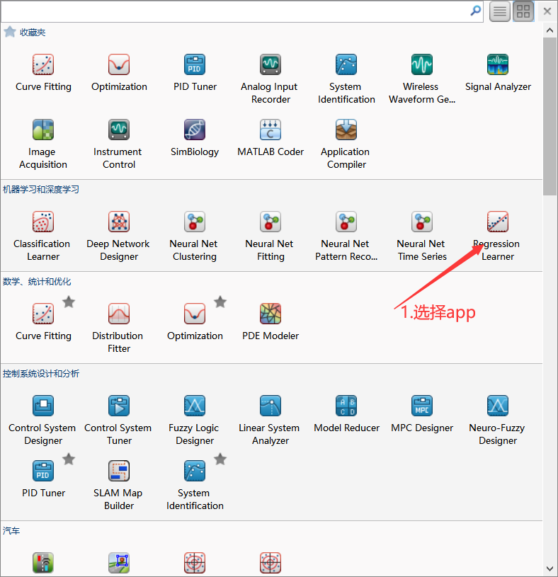
四 APP使用

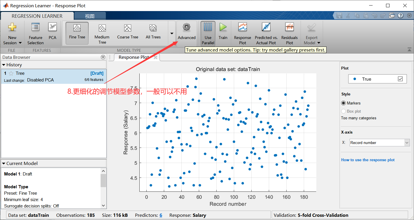
比较适合熟悉基本的模型，但是因为是一个包装好的模型，所以不能调节具体的参数，如果真正的要运行一个模型并且查看和调节各种参数，还是需要自己去写代码来运行。

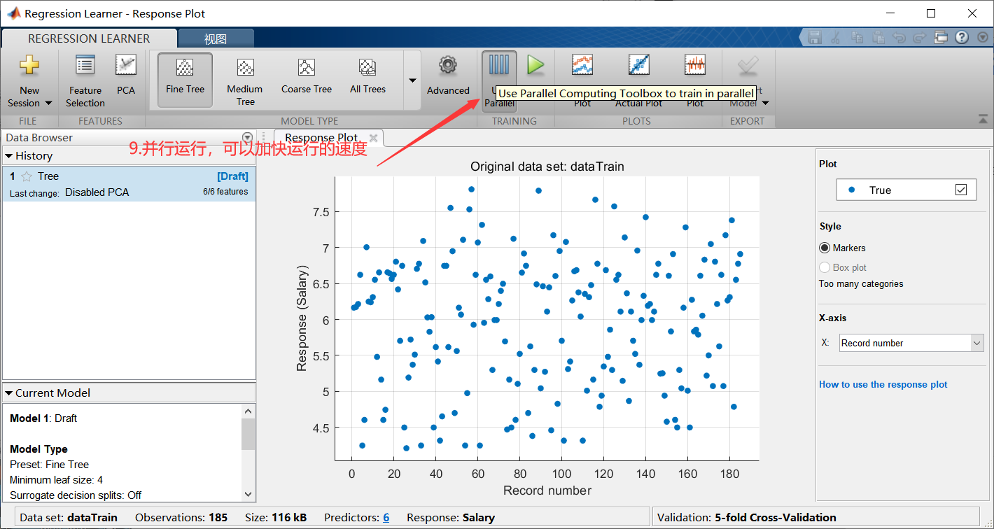
下面是使用APP的具体方法！

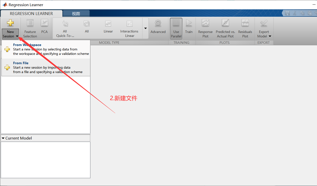
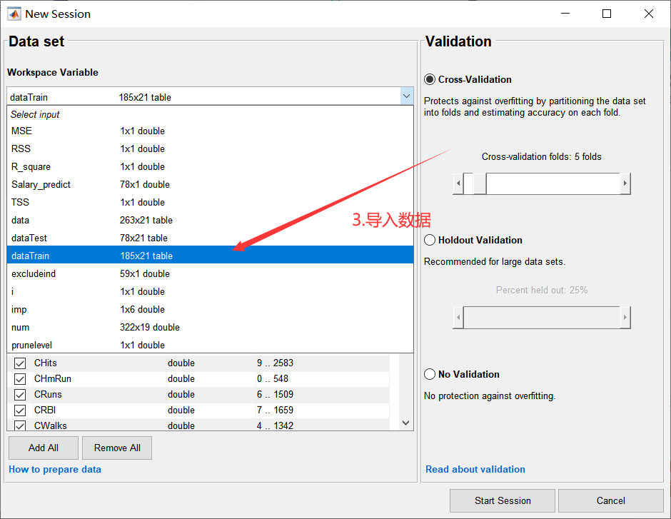
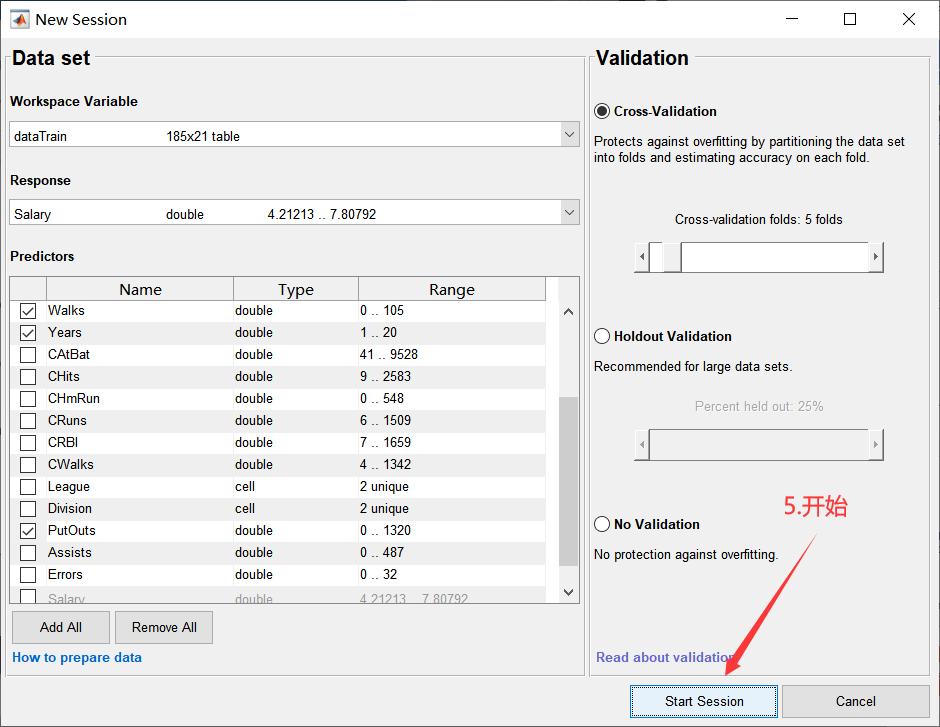
开始后会回到新建界面，如下：

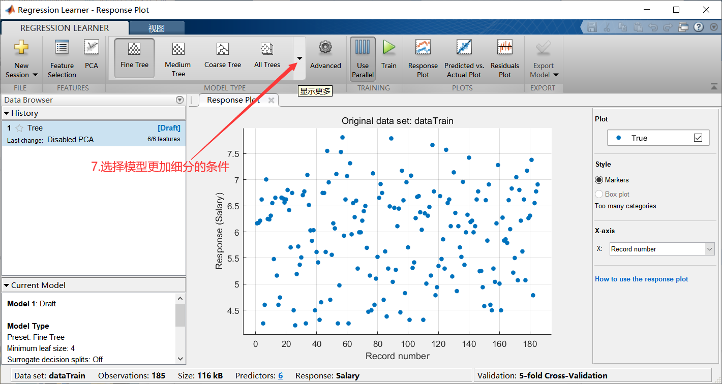
如下所示，也可以贪心一点，全部都选，选择All

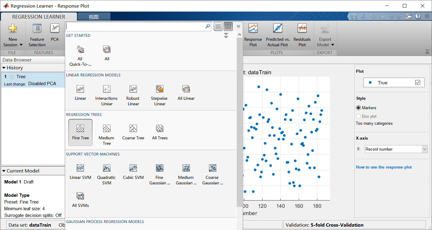
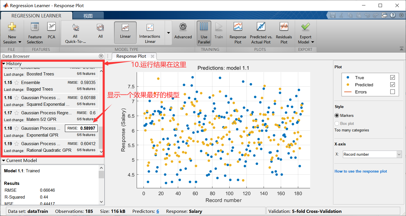
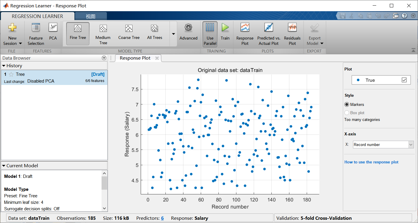
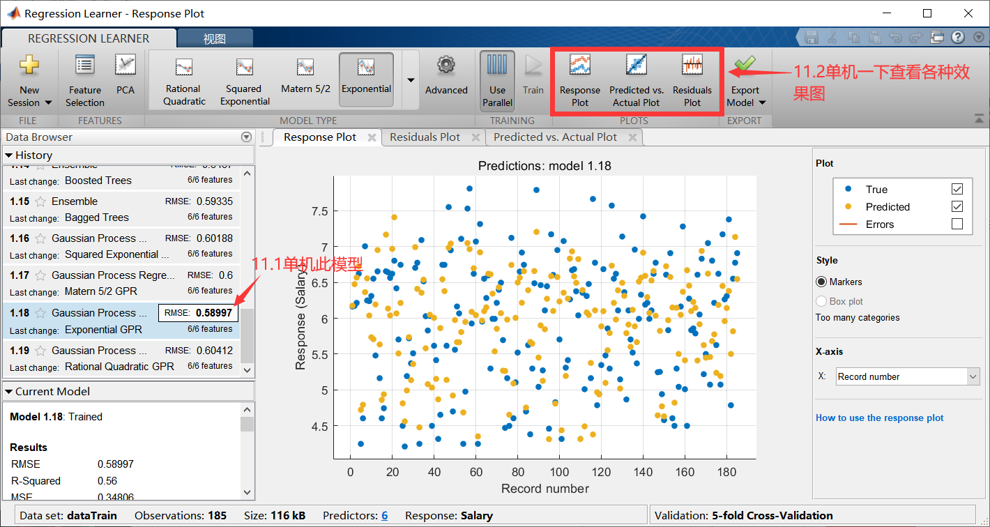
单机任意一个模型之后，可以查看各种效果图：

Original: https://blog.csdn.net/pxyp123/article/details/123425987
Author: pxyp123
Title: 第五课：回归分析