

🔎大家好,我是Sonhhxg_柒,希望你看完之后,能对你有所帮助,不足请指正!共同学习交流🔎
📝个人主页-Sonhhxg_柒的博客_CSDN博客📃
🎁欢迎各位→点赞👍 + 收藏⭐️ + 留言📝
📣系列专栏 – 机器学习【ML】 自然语言处理【NLP】 深度学习【DL】
🖍foreword
✔说明⇢本人讲解主要包括Python、机器学习(ML)、深度学习(DL)、自然语言处理(NLP)等内容。
如果你对这个系列感兴趣的话,可以关注订阅哟👋
介绍
在本课中,您将发现一种使用SVM构建模型的特定方法:支持向量机进行回归,或SVR :支持向量 回归 器。
时间序列中的SVR
在了解 SVR 在时间序列预测中的重要性之前,这里有一些您需要了解的重要概念:
- 回归:监督学习技术,从给定的一组输入中预测连续值。这个想法是在具有最大数据点数的特征空间中拟合一条曲线(或直线)。点击这里了解更多信息。
- 支持向量机 (SVM):一种用于分类、回归和异常值检测的监督机器学习模型。该模型是特征空间中的一个超平面,在分类的情况下充当边界,在回归的情况下充当最佳拟合线。在 SVM 中,通常使用核函数将数据集转换为更高维数的空间,以便它们易于分离。单击此处了解有关 SVM 的更多信息。
- 支持向量回归器 (SVR):一种 SVM,用于找到具有最大数据点数的最佳拟合线(在 SVM 的情况下是超平面)。
为什么选择 SVR?
在上一课中,您了解了 ARIMA,这是一种非常成功的预测时间序列数据的统计线性方法。然而,在许多情况下,时间序列数据具有 非线性,线性模型无法映射。在这种情况下,SVM 考虑回归任务数据中非线性的能力使得 SVR 在时间序列预测中取得成功。
练习 – 建立 SVR 模型
数据准备的前几个步骤与上一课ARIMA的步骤相同。
打开本课中的 /working文件夹,找到 _notebook.ipynb_文件。
- 运行笔记本并导入必要的库:
import sys
sys.path.append('../../')
import os
import warnings
import matplotlib.pyplot as plt
import numpy as np
import pandas as pd
import datetime as dt
import math

from sklearn.svm import SVR
from sklearn.preprocessing import MinMaxScaler
from common.utils import load_data, mape
- 将文件中的数据加载
/data/energy.csv到 Pandas 数据框中并查看: 2
energy = load_data('../../data')[['load']]
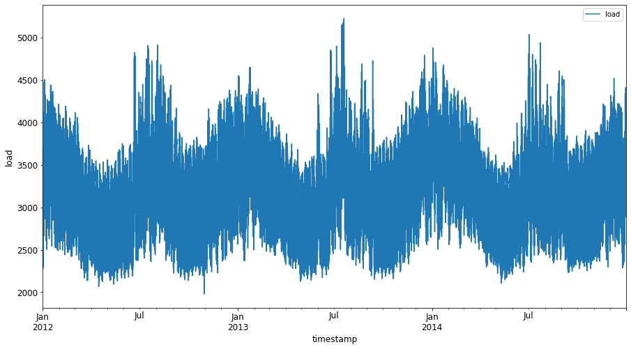
- 绘制从 2012 年 1 月到 2014 年 12 月的所有可用能源数据:2
energy.plot(y='load', subplots=True, figsize=(15, 8), fontsize=12)
plt.xlabel('timestamp', fontsize=12)
plt.ylabel('load', fontsize=12)
plt.show()
创建训练和测试数据集
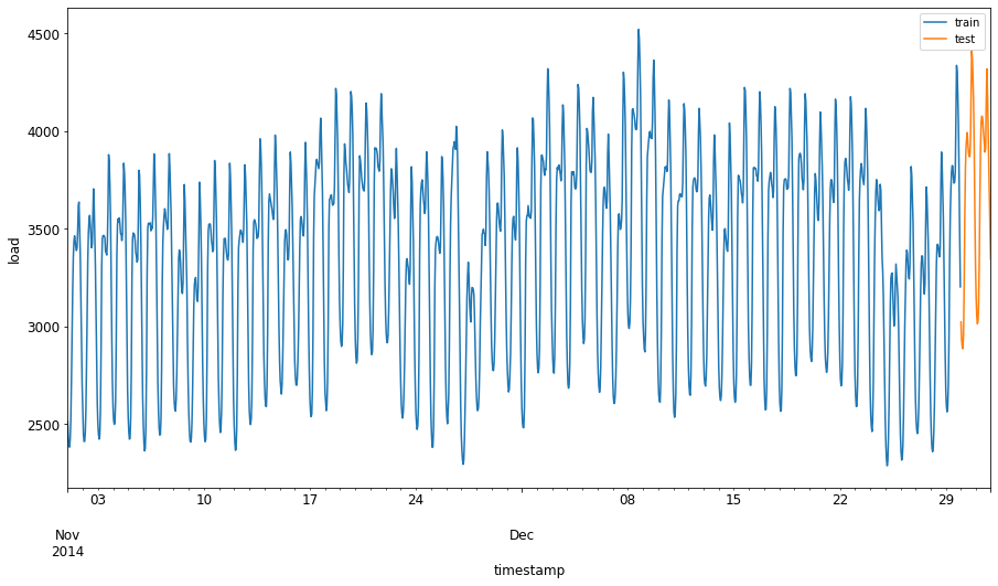
现在您的数据已加载,因此您可以将其分成训练集和测试集。然后,您将重塑数据以创建 SVR 所需的基于时间步长的数据集。您将在训练集上训练您的模型。模型完成训练后,您将评估其在训练集、测试集和完整数据集上的准确性,以查看整体性能。您需要确保测试集覆盖训练集的较晚时间段,以确保模型不会从未来时间段2中获取信息(这种情况称为 过度拟合)。
- 为训练集分配从 2014 年 9 月 1 日到 10 月 31 日两个月的时间段。测试集将包括 2014 年 11 月 1 日至 12 月 31 日这两个月的时间:2
train_start_dt = '2014-11-01 00:00:00'
test_start_dt = '2014-12-30 00:00:00'
- 可视化差异:2
energy[(energy.index < test_start_dt) & (energy.index >= train_start_dt)][['load']].rename(columns={'load':'train'}) \
    .join(energy[test_start_dt:][['load']].rename(columns={'load':'test'}), how='outer') \
    .plot(y=['train', 'test'], figsize=(15, 8), fontsize=12)
plt.xlabel('timestamp', fontsize=12)
plt.ylabel('load', fontsize=12)
plt.show()
准备训练数据
现在,您需要通过对数据执行过滤和缩放来准备训练数据。过滤您的数据集以仅包含您需要的时间段和列,并进行缩放以确保将数据投影在 0,1 区间内。
- 过滤原始数据集以仅包括上述每组时间段,并且仅包括所需的列”负载”加上日期:
train = energy.copy()[(energy.index >= train_start_dt) & (energy.index < test_start_dt)][['load']]
test = energy.copy()[energy.index >= test_start_dt][['load']]

print('Training data shape: ', train.shape)
print('Test data shape: ', test.shape)
Training data shape:  (1416, 1)
Test data shape:  (48, 1)
- 将训练数据缩放到 (0, 1):
scaler = MinMaxScaler()
train['load'] = scaler.fit_transform(train)
- 现在,您缩放测试数据:
test['load'] = scaler.transform(test)
创建具有时间步长的数据
对于 SVR,您将输入数据转换为 [batch, timesteps]. 所以,你重塑了现有的 train_data, test_data这样就有了一个新的维度,它指的是时间步长。
Converting to numpy arrays
train_data = train.values
test_data = test.values
对于这个例子,我们取 timesteps = 5. 因此,模型的输入是前 4 个时间步的数据,输出将是第 5 个时间步的数据。
timesteps=5
使用嵌套列表推导将训练数据转换为 2D 张量:
train_data_timesteps=np.array([[j for j in train_data[i:i+timesteps]] for i in range(0,len(train_data)-timesteps+1)])[:,:,0]
train_data_timesteps.shape
(1412, 5)
将测试数据转换为 2D 张量:
test_data_timesteps=np.array([[j for j in test_data[i:i+timesteps]] for i in range(0,len(test_data)-timesteps+1)])[:,:,0]
test_data_timesteps.shape
(44, 5)
从训练和测试数据中选择输入和输出:
x_train, y_train = train_data_timesteps[:,:timesteps-1],train_data_timesteps[:,[timesteps-1]]
x_test, y_test = test_data_timesteps[:,:timesteps-1],test_data_timesteps[:,[timesteps-1]]

print(x_train.shape, y_train.shape)
print(x_test.shape, y_test.shape)
(1412, 4) (1412, 1)
(44, 4) (44, 1)
实施 SVR
现在,是时候实施 SVR 了。要阅读有关此实现的更多信息,您可以参考此文档。对于我们的实施,我们遵循以下步骤:
- 通过调用
SVR()和传入模型超参数来定义模型:kernel、gamma、c 和 epsilon fit()通过调用函数为训练数据准备模型predict()调用函数进行预测
现在我们创建一个 SVR 模型。这里我们使用RBF 内核,并将超参数 gamma、C 和 epsilon 分别设置为 0.5、10 和 0.05。
model = SVR(kernel='rbf',gamma=0.5, C=10, epsilon = 0.05)
在训练数据上拟合模型1
model.fit(x_train, y_train[:,0])
SVR(C=10, cache_size=200, coef0=0.0, degree=3, epsilon=0.05, gamma=0.5,
kernel=’rbf’, max_iter=-1, shrinking=True, tol=0.001, verbose=False)
进行模型预测1
y_train_pred = model.predict(x_train).reshape(-1,1)
y_test_pred = model.predict(x_test).reshape(-1,1)

print(y_train_pred.shape, y_test_pred.shape)
(1412, 1) (44, 1)
你已经建立了你的 SVR!现在我们需要评估它。
评估您的模型
为了评估,首先我们将数据缩减到原始规模。然后,为了检查性能,我们将绘制原始和预测的时间序列图,并打印 MAPE 结果。
缩放预测和原始输出:
undefined
Scaling the predictions
y_train_pred = scaler.inverse_transform(y_train_pred)
y_test_pred = scaler.inverse_transform(y_test_pred)

print(len(y_train_pred), len(y_test_pred))
Scaling the original values
y_train = scaler.inverse_transform(y_train)
y_test = scaler.inverse_transform(y_test)

print(len(y_train), len(y_test))
检查训练和测试数据的模型性能
我们从数据集中提取时间戳以显示在绘图的 x 轴上。请注意,我们将第一个 timesteps-1值用作第一个输出的输出输入,因此输出的时间戳将在那之后开始。
train_timestamps = energy[(energy.index < test_start_dt) & (energy.index >= train_start_dt)].index[timesteps-1:]
test_timestamps = energy[test_start_dt:].index[timesteps-1:]

print(len(train_timestamps), len(test_timestamps))
1412 44
绘制训练数据的预测:
plt.figure(figsize=(25,6))
plt.plot(train_timestamps, y_train, color = 'red', linewidth=2.0, alpha = 0.6)
plt.plot(train_timestamps, y_train_pred, color = 'blue', linewidth=0.8)
plt.legend(['Actual','Predicted'])
plt.xlabel('Timestamp')
plt.title("Training data prediction")
plt.show()
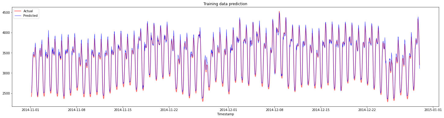
为训练数据打印 MAPE
print('MAPE for training data: ', mape(y_train_pred, y_train)*100, '%')
MAPE for training data: 1.7195710200875551 %
绘制测试数据的预测
plt.figure(figsize=(10,3))
plt.plot(test_timestamps, y_test, color = 'red', linewidth=2.0, alpha = 0.6)
plt.plot(test_timestamps, y_test_pred, color = 'blue', linewidth=0.8)
plt.legend(['Actual','Predicted'])
plt.xlabel('Timestamp')
plt.show()
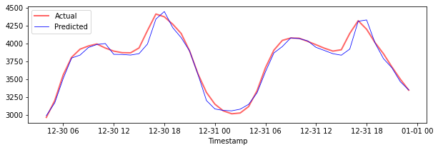
打印 MAPE 用于测试数据
print('MAPE for testing data: ', mape(y_test_pred, y_test)*100, '%')
MAPE for testing data: 1.2623790187854018 %
🏆您在测试数据集上取得了非常好的结果!
检查完整数据集1上的性能
Extracting load values as numpy array
data = energy.copy().values

Scaling
data = scaler.transform(data)

Transforming to 2D tensor as per model input requirement
data_timesteps=np.array([[j for j in data[i:i+timesteps]] for i in range(0,len(data)-timesteps+1)])[:,:,0]
print("Tensor shape: ", data_timesteps.shape)

Selecting inputs and outputs from data
X, Y = data_timesteps[:,:timesteps-1],data_timesteps[:,[timesteps-1]]
print("X shape: ", X.shape,"\nY shape: ", Y.shape)
Tensor shape: (26300, 5)
X shape: (26300, 4)
Y shape: (26300, 1)
undefined
Make model predictions
Y_pred = model.predict(X).reshape(-1,1)

Inverse scale and reshape
Y_pred = scaler.inverse_transform(Y_pred)
Y = scaler.inverse_transform(Y)
plt.figure(figsize=(30,8))
plt.plot(Y, color = 'red', linewidth=2.0, alpha = 0.6)
plt.plot(Y_pred, color = 'blue', linewidth=0.8)
plt.legend(['Actual','Predicted'])
plt.xlabel('Timestamp')
plt.show()
undefined

print('MAPE: ', mape(Y_pred, Y)*100, '%')
MAPE: 2.0572089029888656
🏆非常漂亮的图,显示了一个准确度很高的模型。做得好!
Original: https://blog.csdn.net/sikh_0529/article/details/126961734
Author: Sonhhxg_柒
Title: 【ML】使用支持向量回归器进行时间序列预测
原创文章受到原创版权保护。转载请注明出处:https://www.johngo689.com/626933/
转载文章受原作者版权保护。转载请注明原作者出处!