山东大学人工智能导论实验三 Logistic回归分类器识别猫

目录

【实验目标】

【实验内容】

【数据集介绍】

1.datasets/train_catvnoncat.h5

2.datasets/ test_catvnoncat.h5

3.lr_utils.py中有加载数据集的函数

【代码要求】

定义模型结构

初始化模型的参数

循环

计算当前损失（前向传播）

计算当前梯度（反向传播）

更新参数（梯度下降）

【文档要求】

1.尝试不同的学习率（至少三种），观察不同学习率下随着迭代次数的增加损失值的变化

2.分析不同的学习率对模型准确率的影响及原因，如何选择合适的学习率。

【实验目标】

1. 基于作业二的拓展，进一步理解神经网络的思想
2. 理解逻辑回归实际上是一个非常简单的神经网络

【实验内容】

建立Logistic回归分类器用来识别猫。参考1 和 参考2

【数据集介绍】

1.datasets/train_catvnoncat.h5

保存的是训练集里面的图像数据（本训练集有209张64×64的图像）及对应的分类值（0或1，0表示不是猫，1表示是猫）

2.datasets/ test_catvnoncat.h5

保存的是测试集里面的图像数据（本训练集有50张64×64的图像）及保存的是以bytes类型保存的两个字符串数据，数据为：[b’non-cat’ b’cat’]。

3.lr_utils.py中有加载数据集的函数

【代码要求】

1. 定义模型结构
2. 初始化模型的参数

3. 循环

4. 计算当前损失（前向传播）

5. 计算当前梯度（反向传播）
6. *更新参数（梯度下降）

import numpy as np
import matplotlib.pyplot as plt
import h5py
from lr_utils import load_dataset

train_set_x_orig, train_set_y, test_set_x_orig, test_set_y, classes = load_dataset()

m_train = train_set_y.shape[1]
m_test = test_set_y.shape[1]
num_px = train_set_x_orig.shape[1]

print("训练集的数量: m_train = " + str(m_train))
print("测试集的数量 : m_test = " + str(m_test))
print("每张图片的宽/高 : num_px = " + str(num_px))
print("每张图片的大小 : (" + str(num_px) + ", " + str(num_px) + ", 3)")
print("训练集_图片的维数 : " + str(train_set_x_orig.shape))
print("训练集_标签的维数 : " + str(train_set_y.shape))
print("测试集_图片的维数: " + str(test_set_x_orig.shape))
print("测试集_标签的维数: " + str(test_set_y.shape))

将训练集的维度降低并转置。
train_set_x_flatten = train_set_x_orig.reshape(train_set_x_orig.shape[0], -1).T
将测试集的维度降低并转置。
test_set_x_flatten = test_set_x_orig.reshape(test_set_x_orig.shape[0], -1).T

print("训练集降维最后的维度： " + str(train_set_x_flatten.shape))
print("训练集_标签的维数 : " + str(train_set_y.shape))
print("测试集降维之后的维度: " + str(test_set_x_flatten.shape))
print("测试集_标签的维数 : " + str(test_set_y.shape))

index = 11
plt.imshow(train_set_x_orig[index])
print("y = " + str(train_set_y[:, index]) + ", it's a '" + classes[np.squeeze(train_set_y[:, index])].decode(
    "utf-8") + "' picture.")

train_set_x = train_set_x_flatten / 255
test_set_x = test_set_x_flatten / 255

def sigmoid(z):
    s = 1 / (1 + np.exp(-z))
    return s

def initialize_with_zeros(dim):
    w = np.zeros(shape=(dim, 1))
    b = 0
    # 使用断言来确保我要的数据是正确的
    assert (w.shape == (dim, 1))  # w的维度是(dim,1)
    assert (isinstance(b, float) or isinstance(b, int))  # b的类型是float或者是int

    return (w, b)

def propagate(w, b, X, Y):
    m = X.shape[1]

    # 正向传播
    A = sigmoid(np.dot(w.T, X) + b)
    cost = (- 1 / m) * np.sum(Y * np.log(A) + (1 - Y) * (np.log(1 - A)))

    # 反向传播
    dw = (1 / m) * np.dot(X, (A - Y).T)
    db = (1 / m) * np.sum(A - Y)

    # 使用断言确保我的数据是正确的
    assert (dw.shape == w.shape)
    assert (db.dtype == float)
    cost = np.squeeze(cost)
    assert (cost.shape == ())

    # 创建一个字典，把dw和db保存起来。
    grads = {
        "dw": dw,
        "db": db
    }
    return (grads, cost)

def optimize(w, b, X, Y, num_iterations, learning_rate, print_cost=False):
    costs = []

    for i in range(num_iterations):

        grads, cost = propagate(w, b, X, Y)

        dw = grads["dw"]
        db = grads["db"]

        w = w - learning_rate * dw
        b = b - learning_rate * db

        # 记录成本
        if i % 100 == 0:
            costs.append(cost)
        # 打印成本
        if (print_cost) and (i % 100 == 0):
            print("迭代的次数: %i ， 误差值： %f" % (i, cost))

    params = {
        "w": w,
        "b": b}
    grads = {
        "dw": dw,
        "db": db}
    return (params, grads, costs)

def predict(w, b, X):
    m = X.shape[1]  # 图片的数量
    Y_prediction = np.zeros((1, m))
    w = w.reshape(X.shape[0], 1)

    # 计预测猫在图片中出现的概率
    A = sigmoid(np.dot(w.T, X) + b)
    for i in range(A.shape[1]):
        # 将概率a [0，i]转换为实际预测p [0，i]
        Y_prediction[0, i] = 1 if A[0, i] > 0.5 else 0
    # 使用断言
    assert (Y_prediction.shape == (1, m))

    return Y_prediction

def model(X_train, Y_train, X_test, Y_test, num_iterations=2000, learning_rate=0.5, print_cost=False):
    w, b = initialize_with_zeros(X_train.shape[0])

    parameters, grads, costs = optimize(w, b, X_train, Y_train, num_iterations, learning_rate, print_cost)

    # 从字典"参数"中检索参数w和b
    w, b = parameters["w"], parameters["b"]

    # 预测测试/训练集的例子
    Y_prediction_test = predict(w, b, X_test)
    Y_prediction_train = predict(w, b, X_train)

    # 打印训练后的准确性
    print("训练集准确性：", format(100 - np.mean(np.abs(Y_prediction_train - Y_train)) * 100), "%")
    print("测试集准确性：", format(100 - np.mean(np.abs(Y_prediction_test - Y_test)) * 100), "%")

    d = {
        "costs": costs,
        "Y_prediction_test": Y_prediction_test,
        "Y_prediciton_train": Y_prediction_train,
        "w": w,
        "b": b,
        "learning_rate": learning_rate,
        "num_iterations": num_iterations}
    return d

d = model(train_set_x, train_set_y, test_set_x, test_set_y, num_iterations=2000, learning_rate=0.005, print_cost=True)

绘制图
costs = np.squeeze(d['costs'])
plt.plot(costs)
plt.ylabel('cost')
plt.xlabel('iterations (per hundreds)')
plt.title("Learning rate =" + str(d["learning_rate"]))
plt.show()

learning_rates = [1, 0.01, 0.006, 0.0003, 0.001, 0.0006]
models = {}
for i in learning_rates:
    print("learning rate is: " + str(i))
    models[str(i)] = model(train_set_x, train_set_y, test_set_x, test_set_y, num_iterations=1500, learning_rate=i,
                           print_cost=False)
    print('\n' + "-------------------------------------------------------" + '\n')

for i in learning_rates:
    plt.plot(np.squeeze(models[str(i)]["costs"]), label=str(models[str(i)]["learning_rate"]))

plt.ylabel('cost')
plt.xlabel('iterations')

legend = plt.legend(loc='upper center', shadow=True)
frame = legend.get_frame()
frame.set_facecolor('0.90')
plt.show()

【文档要求】

1.尝试不同的学习率（至少三种），观察不同学习率下随着迭代次数的增加损失值的变化

请粘贴不同学习率下损失的变化曲线图像:

这里我首先打印了一下训练集的内容：

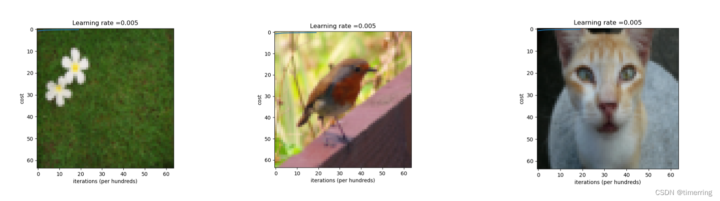
接着对模型进行训练，并打印不同学习率下损失的变化曲线图像：

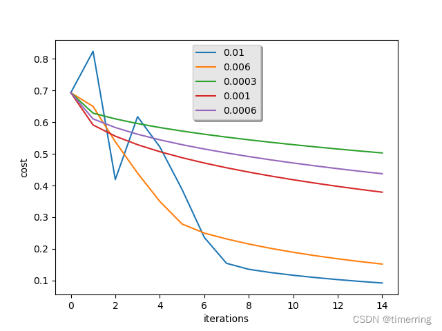
在这里我分析了五种学习率，分别是0.01, 0.006, 0.0003, 0.001, 0.0006，可以看到学习率过低或者过高对于模型的拟合效果都存在一定的影响。当学习率过大则导致模型不收敛，过小则导致模型收敛特别慢或者无法学习。
2.分析不同的学习率对模型准确率的影响及原因，如何选择合适的学习率。

一般在分析选取最优学习率时，可以先采用多个学习率粗略范围的学习率作为尝试，在同一张图上可以看到对应某个区间之间的学习率work best，然后在这个区间内进行较精确的调参，再观察其学习率，是一个不断缩小范围的过程，并且位置不同，对应的合适步长也不同，具体可以使用余弦退火的方式改变学习率的大小，或者以非常低的学习率运行训练，并在每次迭代中线性增加它。当损失功能开始急剧增加时，应停止训练。记录每次迭代的学习速率和损失，最后找到一个合理的学习率。

初学人工智能导论，可能存在错误之处，还请各位不吝赐教。

受于文本原因，本文相关实验工程无法展示出来，现已将资源上传，可自行下载。

山东大学人工智能导论实验3工程文件-Logistic回归分类器识别猫-机器学习文档类资源-CSDN下载山东大学人工智能导论实验3工程文件-Logistic回归分类器识别猫详解博客地址：https://更多下载资源、学习资料请访问CSDN下载频道.https://download.csdn.net/download/m0_52316372/85913095 ;

Original: https://blog.csdn.net/m0_52316372/article/details/125626670
Author: timerring
Title: 山东大学人工智能导论实验三 Logistic回归分类器识别猫