

python 多项式回归以及可视化
简介
多项式回归:回归函数是回归变量多项式的回归1。
令x k x_k x k 为自变量,y y y为因变量:y = f ( x 0 , . . . , x k ) y = f(x_0,…,x_k)y =f (x 0 ,…,x k ) 本文主要介绍两种 一元和 二元
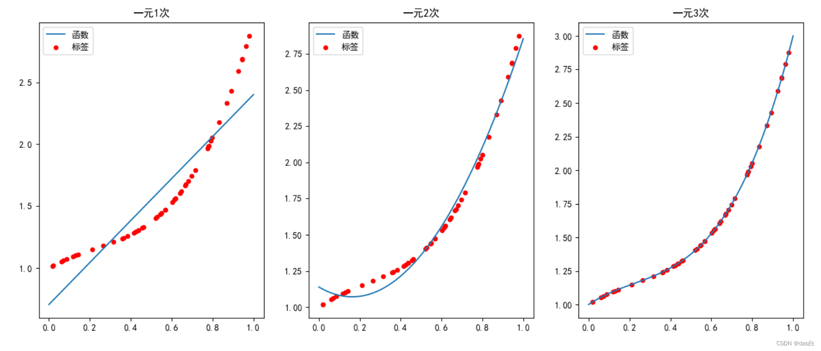
一、一元N次多项式回归
已知数据 x x x 和 y y y,求 b b b 和系数 k k k
公式:y = b + k 1 ∗ x 1 + k 2 ∗ x 2 + . . . + k n ∗ x n y=b + k_1 * x^1 + k_2 * x^2 + … + k_n * x^n y =b +k 1 ∗x 1 +k 2 ∗x 2 +…+k n ∗x n
令方程为:y = 1 + x − 2 ∗ x 2 + 3 ∗ x n y=1 + x -2 * x^2 + 3 * x^n y =1 +x −2 ∗x 2 +3 ∗x n (使用np.random.rand造一些数据,测试多项式回归)
1.1 可视化

; 1.2 代码
代码实现:
import numpy as np
import matplotlib.pyplot as plt
from numpy.linalg import lstsq
plt.rcParams["font.sans-serif"] = ["SimHei"]
plt.rcParams["axes.unicode_minus"] = False

np.random.seed(0)
x_t = np.random.rand(50).reshape(50, -1)
y_t = 1 + x_t + -2 * x_t ** 2 + 3 * x_t ** 3

fig = plt.figure(figsize=(18, 6))
for n in [1, 2, 3]:

    x_tmp = x_t.copy()
    for i in range(2, n+1):
        x_tmp = np.concatenate((x_tmp, x_t ** i), axis=1)
    m = np.ones(x_t.shape)
    m = np.concatenate((m, x_tmp), axis=1)
    k = lstsq(m, y_t, rcond=None)[0].reshape(-1)
    print(k)

    ax = fig.add_subplot(1, 3, n)
    ax.scatter(x_t.reshape(-1), y_t.reshape(-1), c='red', s=20, label='标签')
    x = np.linspace(0, 1, 100)
    y = k[0] + k[1] * x
    for i in range(2, n+1):
        y += k[i] * (x ** i)
    ax.plot(x, y, label='函数')
    ax.set_title('一元' + str(n) + '次')
    ax.legend()

plt.legend()

plt.show()
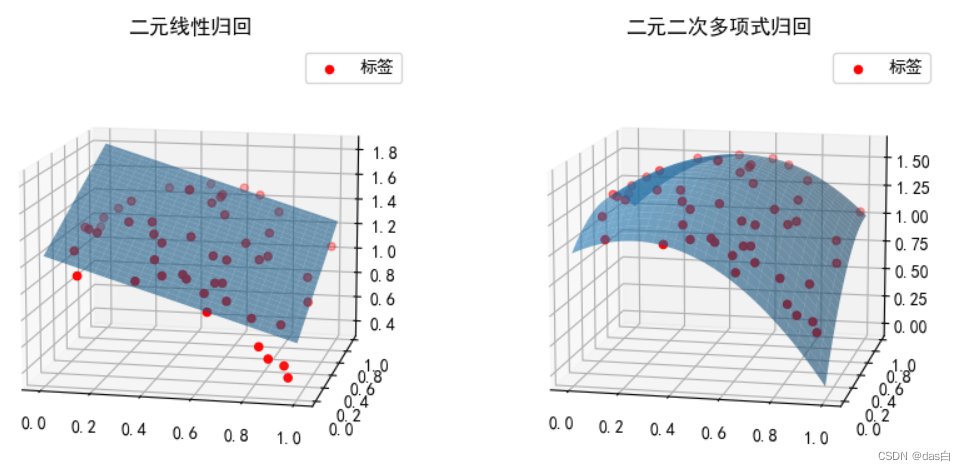
二、二元二次多项式回归
已知数据 x 1 x_1 x 1 、x 2 x_2 x 2 和 y y y,求 b b b 和系数 k k k
公式:y = b + k 1 ∗ x 1 + k 2 ∗ x 1 2 + k 3 ∗ x 2 + k 4 ∗ x 2 2 + k 5 ∗ x 1 ∗ x 2 y=b + k_1 * x_1 + k_2 * x_1^2 + k_3 * x_2 + k_4 * x_2^2 + k_5 * x_1 * x_2 y =b +k 1 ∗x 1 +k 2 ∗x 1 2 +k 3 ∗x 2 +k 4 ∗x 2 2 +k 5 ∗x 1 ∗x 2
令方程为:y = 1 + x 1 − 2 ∗ x 1 2 + x 2 − x 2 2 + x 1 ∗ x 2 y=1 + x_1 -2 * x_1^2 + x_2 -x_2^2 + x_1*x_2 y =1 +x 1 −2 ∗x 1 2 +x 2 −x 2 2 +x 1 ∗x 2 (使用np.random.rand造一些数据,测试多项式回归)
2.1 可视化
; 2.2 代码
代码实现:2
import numpy as np
import matplotlib.pyplot as plt
from numpy.linalg import lstsq
plt.rcParams["font.sans-serif"] = ["SimHei"]
plt.rcParams["axes.unicode_minus"] = False

np.random.seed(0)
x_1 = np.random.rand(50).reshape(50, -1)
x_2 = np.random.rand(50).reshape(50, -1)
y_t = 1 + x_1 + -2 * x_1 ** 2 + x_2 + -1 * x_2 ** 2 + x_1*x_2

fig = plt.figure(figsize=(10, 5))
m = np.ones(x_1.shape)
m = np.hstack((m, x_1, x_1 ** 2, x_2, x_2 ** 2, x_1*x_2))
k = lstsq(m, y_t, rcond=None)[0].reshape(-1)
print(k)

ax = fig.add_subplot(1, 2, 2, projection='3d')
ax.scatter(x_1.reshape(-1), x_2.reshape(-1), y_t.reshape(-1), c='red', s=20, label='标签')
x1 = np.linspace(0, 1, 100)
x2 = np.linspace(0, 1, 100)
x, y =np.meshgrid(x1, x2)
z = k[0] + k[1] * x + k[2] * x ** 2 + k[3] * y + k[4] * y**2 + k[5] * x * y
ax.plot_surface(x, y, z,rstride=4,cstride=4,alpha=0.6)
ax.legend()
ax.set_title('二元二次多项式归回')
ax.view_init(12,-78)

ax = fig.add_subplot(1, 2, 1, projection='3d')
ax.scatter(x_1.reshape(-1), x_2.reshape(-1), y_t.reshape(-1), c='red', s=20, label='标签')
m = np.ones(x_1.shape)
m = np.hstack((m, x_1, x_2))
k = lstsq(m, y_t, rcond=None)[0].reshape(-1)
print(k)
x1 = np.linspace(0, 1, 100)
x2 = np.linspace(0, 1, 100)
x, y =np.meshgrid(x1, x2)
z = k[0] + k[1] * x + k[2] * y
ax.plot_surface(x, y, z,rstride=4,cstride=4,alpha=0.6)
ax.legend()
ax.set_title('二元线性归回')
ax.view_init(12,-78)

plt.show()
Original: https://blog.csdn.net/qq_38204686/article/details/126276228
Author: 大米粥哥哥
Title: python 多项式回归以及可视化
原创文章受到原创版权保护。转载请注明出处:https://www.johngo689.com/626643/
转载文章受原作者版权保护。转载请注明原作者出处!