

逻辑回归(Logistic Regression)是一种分类算法。不同于线性回归的回归属性,逻辑回归是的输出是一组离散值。以最简单的二元分类为例,逻辑回归通过每个样本的特征和其相应权重的相乘之后,通过sigmoid函数来得到相应的(0,1)值。如上所述,逻辑回归的预测函数为g ( x ) = 1 1 + e − z g(x)=\frac{1}{1+e^{-z}}g (x )=1 +e −z 1 ,其中z = W T X z=W^{T}X z =W T X,W,X分别为我们要求的权重和特征向量。之所以用Sigmoid函数是因为Sigmoid函数良好的性质,如图
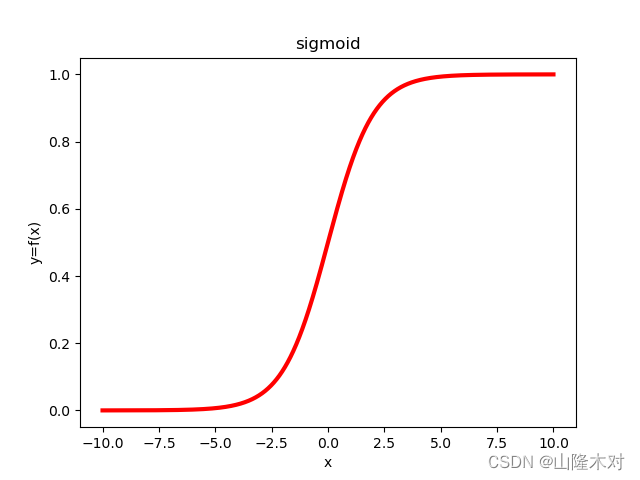

因为Sigmoid函数可以将(-∞,+∞)上的值映射到(0,1)区间,因此,Sigmoid输出也可以表示一种概率,即,p ( y = 1 ∣ W , X ) = 1 1 + e − W T X p(y=1|W,X)=\frac{1}{1+e^{-W^{T}X}}p (y =1 ∣W ,X )=1 +e −W T X 1 ,p ( y = 0 ∣ W , X ) = 1 − p ( y = 1 ∣ W , X ) p(y=0|W,X)=1-p(y=1|W,X)p (y =0 ∣W ,X )=1 −p (y =1 ∣W ,X )。
所以对一个样本预测正确的概率为p ( r i g h t ) = p ( y = 1 ) y i ∗ p ( y = 0 ) 1 − y i p(right)=p(y=1)^{y_{i}}*p(y=0)^{1-y_{i}}p (r i g h t )=p (y =1 )y i ∗p (y =0 )1 −y i 。
我们希望这个预测的正确率达到最大,可以用极大似然函数来进行求解。即
l n ( L ( θ ) ) = ∑ i = 1 m y i l n ( g ( θ T X ) ) + ( 1 − y i ) l n ( 1 − g ( θ T X ) ) ln(L(\theta))=\sum^{m}{i=1}{y{i}ln(g(\theta^{T}X))+(1-y_{i})ln(1-g(\theta^{T}X))}l n (L (θ))=i =1 ∑m y i l n (g (θT X ))+(1 −y i )l n (1 −g (θT X ))我们期望对每个样本的估计值的正确率都能够达到最大,即对极大似然函数求其极大值。其间,在函数值优化过程中,我们习惯用最小化,因此在极大似然函数前面加一个负号.
根据西瓜书所说(证明),上述函数是凸函数,因此可以用牛顿法或者梯度下降法对齐进行求解。
因此,即为我们所求的目标函数。为求其最(极)小值,对其求梯度。
∂ J ∂ θ = − ∑ i = 1 m ( y i − g ( θ T X i ) ) X i \frac{\partial J}{\partial \theta}=-\sum^{m}{i=1}{(y{i}-g(\theta^{T}X_{i}))X_{i}}∂θ∂J =−i =1 ∑m (y i −g (θT X i ))X i
(敲公式太麻烦,直接给结果了)
笔者使用直球梯度下降法对数据集进行求解。所选用的数据集为线性分布的二维样本点,并且其标签为(0,1)二元值。
; 数据处理
data=pd.read_csv("data1.csv",header=None)
data=data.values
labels=data[:,-1]
labels=(labels+1)/2
feature=data[:,:-1]

len=feature.shape[0]
要是有人看,需要数据集的话就留个言吧
梯度下降
注意这里将梯度下降的过程分解一下,方便debug,然后毕竟数据量少,就用最原始的梯度下降法了,不搞那些奇淫巧技了
def GDescent(train_data,train_label,coeffience,alpha=0.1):
    m=train_data.shape[0]
    if(m==train_label.shape[0]):

        step1=1/(1+np.exp(-np.dot(coeffience,train_data.T)))
        step2=step1-train_label
        step3=np.multiply(step2,train_data.T).T
        step4=np.sum(step3,axis=0)/m
        differential_array=step4

        differential_array=differential_array.T

        coeffience=coeffience-alpha*differential_array

        return coeffience
    pass
预测函数
def PreCal(train_data,coeffience):
    test_pre=1/(1+np.exp(-np.dot(coeffience,train_data.T)))

    return test_pre
误差求解
def DistanceCal(test_pre,train_label):
    m=test_pre.shape[0]
    if(m==train_label.shape[0]):
        distance=np.sum(np.abs(test_pre-train_label)/m)
        return distance
初始化参数及求解
因为数据集是线性可分的,且
feature_dim=feature.shape[1]
coeffience=np.ones(feature_dim)
distance_e=1e-3
test_pre=np.zeros(labels.shape[0])
distance=DistanceCal(test_pre,labels)
coeffiences=[]
start=time()
while(distance>distance_e):
coeffiences.append(coeffience)
coeffience=GDescent(feature,labels,coeffience)
test_pre=PreCal(feature,coeffience)
distance=DistanceCal(test_pre,labels)
print("The current coeffience is ",coeffience)
print("The current distance is ",distance)
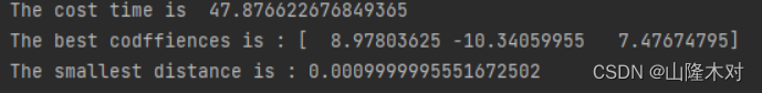
print("The cost time is ",time()-start)
print("The best codffiences is :",coeffiences[-1])
print("The smallest distance is :",distance)
画图
data_plus_x=[]
data_plus_y=[]
data_minus_x=[]
data_minus_y=[]
for i in range(data.shape[0]):
if data[i][-1]==1:
data_plus_x.append(data[i][1])
data_plus_y.append(data[i][2])
if data[i][-1]==-1:
data_minus_x.append(data[i][1])
data_minus_y.append(data[i][2])
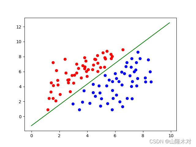
pyplot.scatter(data_plus_x,data_plus_y,c="r")
pyplot.scatter(data_minus_x,data_minus_y,c="b")
x=np.arange(0,10,0.1)
y=(-coeffience[0]-coeffience[1]*x)/coeffience[2]
pyplot.plot(x,y,c="g")
pyplot.show()
结果和图
GPU版本
之后,早就听说一种可以使用GPU的掌法,遂想试一试,使用的是numba的cuda库,对于没有cuda C++编程经验的人来讲,接口也相对比较简单,容易上手。CudaAPI。
和CPU处理不同,GPU主要做一些大量的并行简单运算,因此,需要先为执行的数据分配GPU,并且指定其中的Grid、Block、Thread数量。直接上代码
from numba import cuda
import pandas as pd
from math import exp,fabs,ceil
import numpy as np
from time import time
from matplotlib import pyplot
data=pd.read_csv("data1.csv",header=None)
data=data.values
labels=data[:,-1]
labels=(labels+1)/2
features=data[:,:-1]
distance_e=1e-3
result=cuda.device_array([features.shape[0],features.shape[1]])
test_pre_gpu=cuda.device_array(labels.shape[0])
distances_gpu=cuda.device_array(labels.shape[0])
thread_per_block_2D=(16,16)
block_per_grid_x=ceil(features.shape[0]/thread_per_block_2D[0])
block_per_grid_y=ceil(features.shape[1]/thread_per_block_2D[1])
block_per_grid_2D=(block_per_grid_x,block_per_grid_y)
thread_per_block=128
block_per_grid=ceil(features.shape[0]*features.shape[1]/thread_per_block)
m=features.shape[0]

@cuda.jit()
def GDescent(train_data,train_label,coeffience,result):

    idx,idy=cuda.grid(2)
    if idx<train_data.shape[0] and idy <train_data.shape[1]:
        tmp=0
        for i in range(coeffience.shape[0]):
            tmp+=-coeffience[i]*train_data[idx][i]

        result[idx][idy]=(1/(1+exp(tmp))-train_label[idx])*train_data[idx][idy]

@cuda.jit()
def PreCal(train_data,coeffience,test_pre):
    idx=cuda.threadIdx.x+cuda.blockIdx.x*cuda.blockDim.x
    idy=cuda.threadIdx.y+cuda.blockIdx.y*cuda.blockDim.y
    if idx<train_data.shape[0] and idy<train_data.shape[1]:
        tmp=0
        for i in range(coeffience.shape[0]):
            tmp+=-coeffience[i]*train_data[idx][i]
        test_pre[idx]=1/(1+exp(tmp))

@cuda.jit()
def DistanceCal(test_pre,train_label,distances):
    idx=cuda.threadIdx.x+cuda.blockIdx.x*cuda.blockDim.x
    if idx<test_pre.shape[0]:
        distances[idx]=fabs(test_pre[idx]-train_label[idx])

coeffiences=[]
distance=1
coeffience=np.ones(features.shape[1])
test_pre=0
alpha=0.1

start=time()
while(distance>distance_e):
    coeffiences.append(coeffience)
    GDescent[block_per_grid_2D, thread_per_block_2D](features, labels, coeffience, result)
    cuda.synchronize()
    gradient = np.sum(result.copy_to_host(), axis=0) / m
    coeffience=coeffience-alpha*gradient
    PreCal[block_per_grid,thread_per_block](features,coeffience,test_pre_gpu)
    cuda.synchronize()
    test_pre=test_pre_gpu.copy_to_host()
    DistanceCal[block_per_grid,thread_per_block](test_pre,labels,distances_gpu)
    cuda.synchronize()
    distances=distances_gpu.copy_to_host()
    distance=np.sum(distances)/m
    print("The current coeffience is ",coeffience)
    print("The current distance is ",distance)
print("The GPU cost time is",time()-start)

print("The best coeffience is :",coeffiences[-1])
print("The smallest distance is :",distance)

data_plus_x=[]
data_plus_y=[]
data_minus_x=[]
data_minus_y=[]

for i in range(data.shape[0]):
    if data[i][-1]==1:
        data_plus_x.append(data[i][1])
        data_plus_y.append(data[i][2])
    if data[i][-1]==-1:
        data_minus_x.append(data[i][1])
        data_minus_y.append(data[i][2])

pyplot.scatter(data_plus_x,data_plus_y,c="r")
pyplot.scatter(data_minus_x,data_minus_y,c="b")
x=np.arange(0,10,0.1)
y=(-coeffience[0]-coeffience[1]*x)/coeffience[2]
pyplot.plot(x,y,c="g")
pyplot.show()
最后结果如下
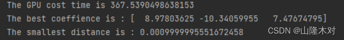

可以看到最后求出的权重和CPU版本是一样的,但是时间远不如想象中的理想,原因如下:
1)在CPU版本中,使用了Numpy库,numpy在底层性能上已经可以说是优化到极致了。
2)使用GPU计算的逻辑是,由于GPU的memory比较小,因此需要将数据先从CPU拷贝到GPU,计算之后再将结果返回,因此会产生通信代价。
但是我看过其他博主写过的文章里用numba.cuda处理1200W数据量的样本时,花费的时间确实要比CPU要小很多。也就是当数据量达到一定规模时,GPU计算的优势才能够得以体现。
Original: https://blog.csdn.net/lyx369639/article/details/125309643
Author: 山隆木对
Title: Logistic Regression逻辑回归函数Python实现
原创文章受到原创版权保护。转载请注明出处:https://www.johngo689.com/623029/
转载文章受原作者版权保护。转载请注明原作者出处!