

文章目录
- 摘要
- 一、简介
- 二、扩散过程
* - 2.1 定义扩散过程
- 2.2 重参数技巧得到迭代公式
- 2.3 得到全局扩散公式
- 2.4 扩散过程实现代码
– - 三、逆扩散过程
* - 3.1 目标公式
- 3.2 后验条件概率
- 四、优化目标
* - 4.1 损失函数公式推导
- 4.2 损失函数代码实现
- 五、算法流程
* - 5.1 模型训练代码
- 5.2 模型采样代码
- 5.3 训练好的模型效果
摘要
The diffusion model is a generative model of the Encoder-Decoder architecture, which is divided into a diffusion stage and an inverse diffusion stage. In the diffusion stage, by continuously adding noise to the original data, the data is changed from the original distribution to the distribution we expect, for example, the original data distribution is changed to a normal distribution by continuously adding Gaussian noise. During the inverse diffusion stage, a neural network is used to restore the data from a normal distribution to the original data distribution. Its advantage is that each point on the normal distribution is a mapping of the real data, and the model has better interpretability. The disadvantage is that iterative sampling is slow, resulting in low model training and prediction efficiency.
扩散模型是Encoder-Decoder架构的生成模型,分为扩散阶段和逆扩散阶段。 在扩散阶段,通过不断对原始数据添加噪声,使数据从原始分布变为我们期望的分布,例如通过不断添加高斯噪声将原始数据分布变为正态分布。 在逆扩散阶段,使用神经网络将数据从正态分布恢复到原始数据分布。 它的优点是正态分布上的每个点都是真实数据的映射,模型具有更好的可解释性。 缺点是迭代采样速度慢,导致模型训练和预测效率低。
一、简介
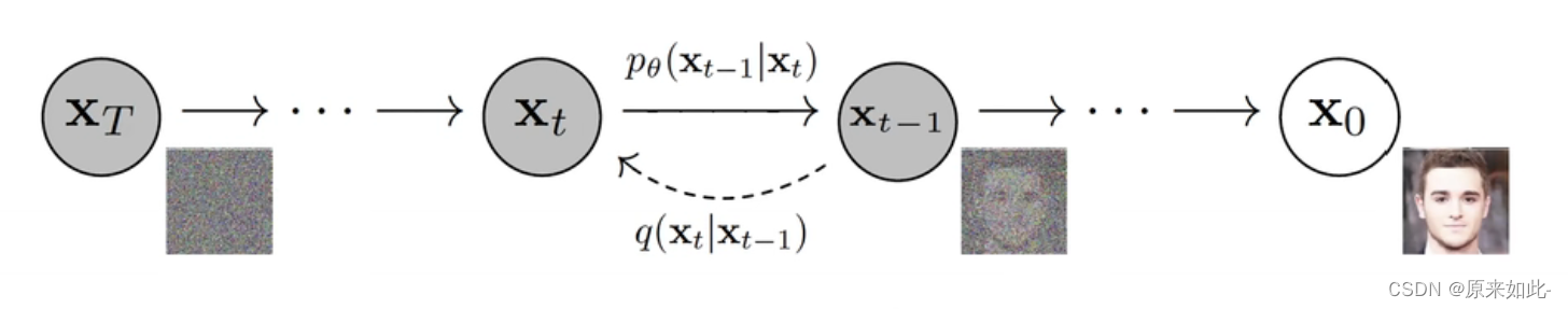
Diffusion model模型分为扩散过程和逆扩散过程,扩散过程通过对原始数据不断加入高斯噪音,使原始数据变为高斯分布的数据,即从X 0 X_0 X 0 − > ->−> X T X_T X T 。逆扩散过程通过高斯噪声还原出图片,即从X T X_T X T − > ->−> X 0 X_0 X 0 。

; 二、扩散过程
2.1 定义扩散过程
在设定扩散过程是一个马尔可夫链的条件下,向原始信息中不断添加高斯噪声,每一步添加高斯噪声的过程是从X t − 1 − > X t X_{t-1} -> X_t X t −1 −>X t ,于是定义公式:
q ( x t ∣ x t − 1 ) = N ( x t ; 1 − β t x t − 1 , β t I ) q(x_t|x_{t-1}) = N(x_t;\sqrt{1-\beta_t}x_{t-1} ,\beta_tI)q (x t ∣x t −1 )=N (x t ;1 −βt x t −1 ,βt I )
该公式表示从x t − 1 − > x t x_{t-1}->x_t x t −1 −>x t 是一个以1 − β t x t − 1 \sqrt{1-\beta_t}x_{t-1}1 −βt x t −1 为均值β t \beta_t βt 为方差的高斯分布变换。
2.2 重参数技巧得到迭代公式
利用重参数技巧得到每一次添加高斯噪声的公式如下:
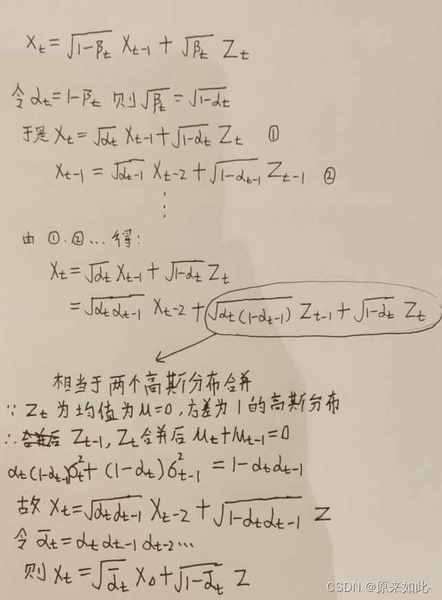
X t = 1 − β t X t − 1 + β t Z t X_t = \sqrt{1-\beta_t}X_{t-1} + \sqrt{\beta}_tZ_t X t =1 −βt X t −1 +βt Z t
- X t X_t X t 表示 t 时刻的数据分布
- Z t Z_t Z t 表示 t 时刻添加的高斯噪音,一般固定是均值为0方差为1的高斯分布
- 1 − β t X t − 1 \sqrt{1-\beta_t}X_{t-1}1 −βt X t −1 表示当前时刻分布的均值
- β t \sqrt{\beta}_t βt 表示当前时刻分布的标准差(标准差=方 差 \sqrt{方差}方差)
注意:其中β t \beta_t βt 是预先设定0~1之间的常量,故扩散过程不含参。
2.3 得到全局扩散公式
在 2.2的迭代公式中可知,扩散过程中只有一个参数β \beta β,而β \beta β是预先设置的常量,故扩散过程中无未知的需要学习的参数,所以只需要知道初始数据分布X 0 X_0 X 0 和β t \beta_t βt 就可以得到任意时刻的分布X t X_t X t ,具体公式如下:
- X 0 X_0 X 0 为原始数据的分布
- α t = 1 − β t \alpha_t = 1 – \beta_t αt =1 −βt
- α t ˉ = ∏ i = 1 t α i \bar{\alpha_t} = \prod_{i=1}^{t}\alpha_i αt ˉ=∏i =1 t αi
- Z为均值为0方差为1的高斯分布
; 2.4 扩散过程实现代码
2.4.1 总结扩散公式
由 2.3可知扩散过程公式为:
X t = α t ˉ X 0 + 1 − α ˉ Z X_t = \sqrt{\bar{\alpha_t}}X_0 + \sqrt{1 – \bar{\alpha}}Z X t =αt ˉX 0 +1 −αˉZ其中:
- X 0 X_0 X 0 为原始数据的分布
- α t = 1 − β t \alpha_t = 1 – \beta_t αt =1 −βt
- α t ˉ = ∏ i = 1 t α i \bar{\alpha_t} = \prod_{i=1}^{t}\alpha_i αt ˉ=∏i =1 t αi
- Z为均值为0方差为1的高斯分布
2.4.2 代码
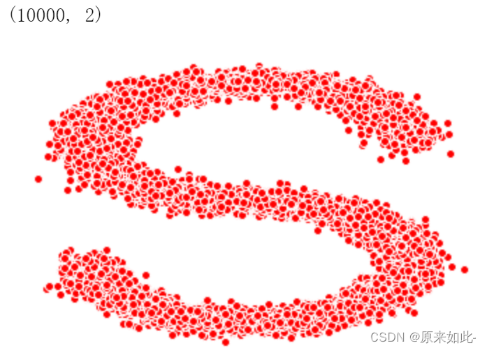
- 用make_s_curve生成数据为例得到X 0 X_0 X 0
s_curve, _ = make_s_curve(10**4, noise=0.1)
x_0 = s_curve[:, [0, 2]]/10.0

print(np.shape(x_0))

data = x_0.T
fig, ax = plt.subplots()
ax.scatter(*data, color='red', edgecolor='white')
ax.axis('off')
dataset = torch.Tensor(data)
2. 假定有100个时刻设置, 所有时刻的β \beta β
num_steps = 100
betas = torch.linspace(-6, 6, num_steps)
betas = torch.sigmoid(betas)*(0.5e-2 - 1e-5)+1e-5
β \beta β为0-1之前很小的数,最大值为0.5e-2,最小值为1e-5
3. 得到α \alpha α(α = 1 − β \alpha = 1 – \beta α=1 −β)
alphas = 1 - betas
- 得到各个时刻的α t ˉ \bar{\alpha_t}αt ˉ(α t ˉ = ∏ i = 1 t α i \bar{\alpha_t} = \prod_{i=1}^{t}\alpha_i αt ˉ=∏i =1 t αi )
alphas_prod = torch.cumprod(alphas, 0)
- 得到α t \sqrt{\alpha_t}αt
alphas_bar_sqrt = torch.sqrt(alphas_bar)
- 得到1 − α t ˉ \sqrt{1-\bar{\alpha_t}}1 −αt ˉ
one_minus_alphas_bar_sqrt = torch.sqrt(1-alphas_bar)
- 输入X 0 X_0 X 0 与时刻t,得到X t X_t X t ,即X t = α t ˉ X 0 + 1 − α t ˉ Z X_t = \sqrt{\bar{\alpha_t}}X_0 + \sqrt{1 – \bar{\alpha_t}}Z X t =αt ˉX 0 +1 −αt ˉZ
def x_t(x_0, t):
    noise = torch.randn_like(x_0)
    return (alphas_bar_sqrt[t]*x_0 + one_minus_alphas_bar_sqrt[t]*noise)
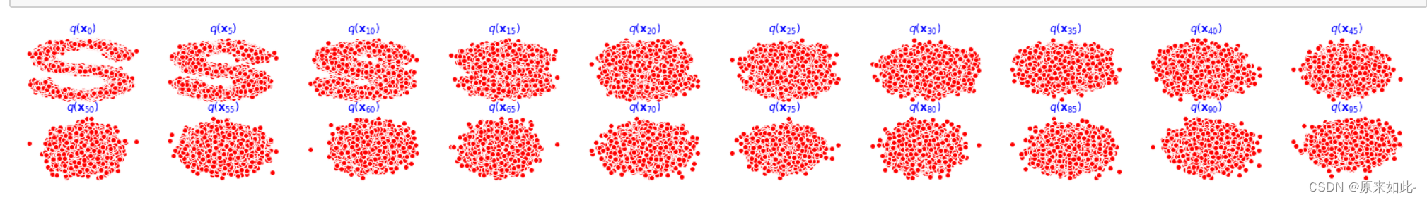
- 扩散过程演示
num_shows = 20
fig, axs = plt.subplots(2, 10, figsize=(28, 3))
plt.rc('text', color='blue')

for i in range(num_shows):
    j = i//10
    k = i%10
    num_x_t = x_t(dataset, torch.tensor([i*num_steps//num_shows]))
    axs[j, k].scatter(*num_x_t, color='red', edgecolor='white')
    axs[j, k].set_axis_off()
    axs[j, k].set_title('$q(\mathbf{x}_{'+str(i*num_steps//num_shows)+'})$')
三、逆扩散过程
3.1 目标公式
扩散过程是将原始数据不断加噪得到高斯噪声,逆扩散过程是从高斯噪声中恢复原始数据,我们假定逆扩散过程仍然是一个马尔可夫链的过程,要做的是X T − > X 0 X_T->X_0 X T −>X 0 ,用公式表达如下:
p θ ( x t − 1 ∣ x t ) = N ( x t − 1 ; u θ ( x t , t ) , Σ θ ( x t , t ) ) p_\theta(x_{t-1}|x_t) = N(x_{t-1}; u_\theta(x_t, t),\Sigma_\theta(x_t, t) )p θ(x t −1 ∣x t )=N (x t −1 ;u θ(x t ,t ),Σθ(x t ,t ))
3.2 后验条件概率
推导得到后验条件概率q ( x t − 1 ∣ x t , x 0 ) q(x_{t-1}|x_t, x_0)q (x t −1 ∣x t ,x 0 )

其方差β t ˉ \bar{\beta_t}βt ˉ为:
β t ˉ = 1 − α t − 1 ˉ 1 − α t ˉ β t \bar{\beta_t} = \frac{1-\bar{\alpha_{t-1}}}{1-\bar{\alpha_t}}\beta_t βt ˉ=1 −αt ˉ1 −αt −1 ˉβt
均值u ˉ ( x t − 1 , x 0 ) \bar{u}(x_{t-1}, x_0)u ˉ(x t −1 ,x 0 )为:
u ˉ ( x t − 1 , x 0 ) = α t ( 1 − α ˉ t − 1 ) 1 − α t ˉ x t + α ˉ t − 1 β t 1 − α t ˉ x 0 \bar{u}(x_{t-1}, x_0)=\frac{\sqrt{\alpha_t}(1-\bar{\alpha}{t-1})}{1-\bar{\alpha_t}}x_t+\frac{\sqrt{\bar{\alpha}{t-1}}\beta_t}{1-\bar{\alpha_t}}x_0 u ˉ(x t −1 ,x 0 )=1 −αt ˉαt (1 −αˉt −1 )x t +1 −αt ˉαˉt −1 βt x 0
逆扩散过程模型不应当事先知道x 0 x_0 x 0 ,故需将x 0 x_0 x 0 用x t x_t x t 代替,根据
2.4得到: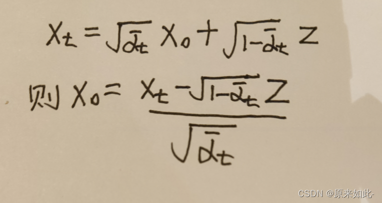
代入均值公式中,化简后得到后验条件均值:
u ˉ t = 1 α t ( x t − β t 1 − α t ˉ z t ) \bar{u}_t=\frac{1}{\sqrt{\alpha_t}}(x_t-\frac{\beta_t}{\sqrt{1-\bar{\alpha_t}}}z_t)u ˉt =αt 1 (x t −1 −αt ˉβt z t )
; 四、优化目标
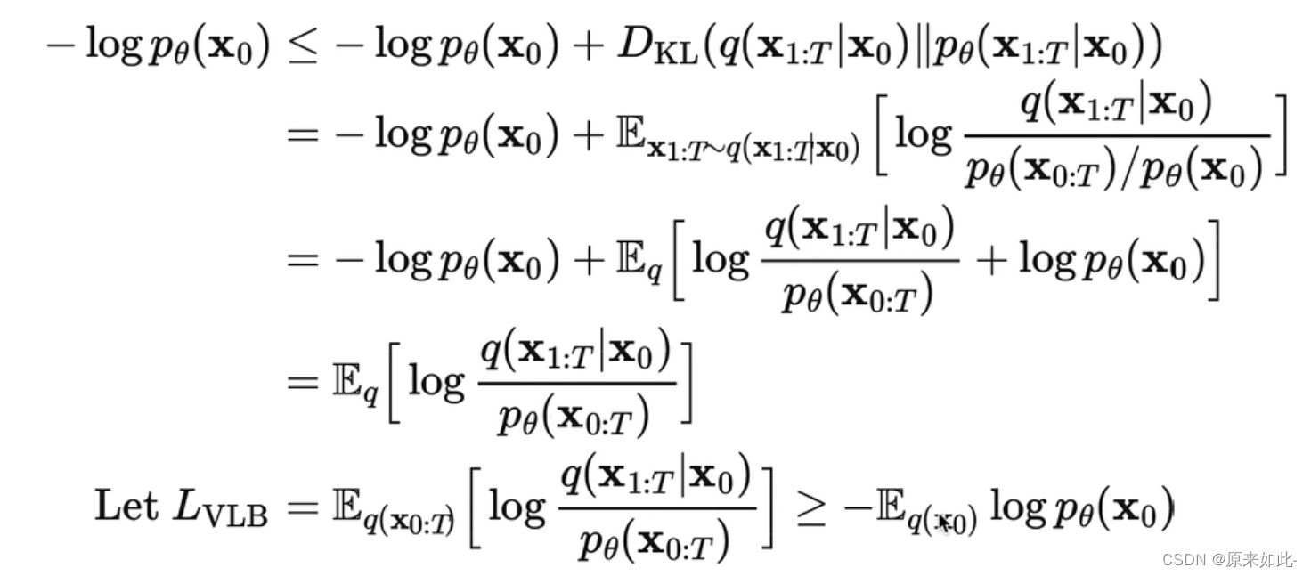
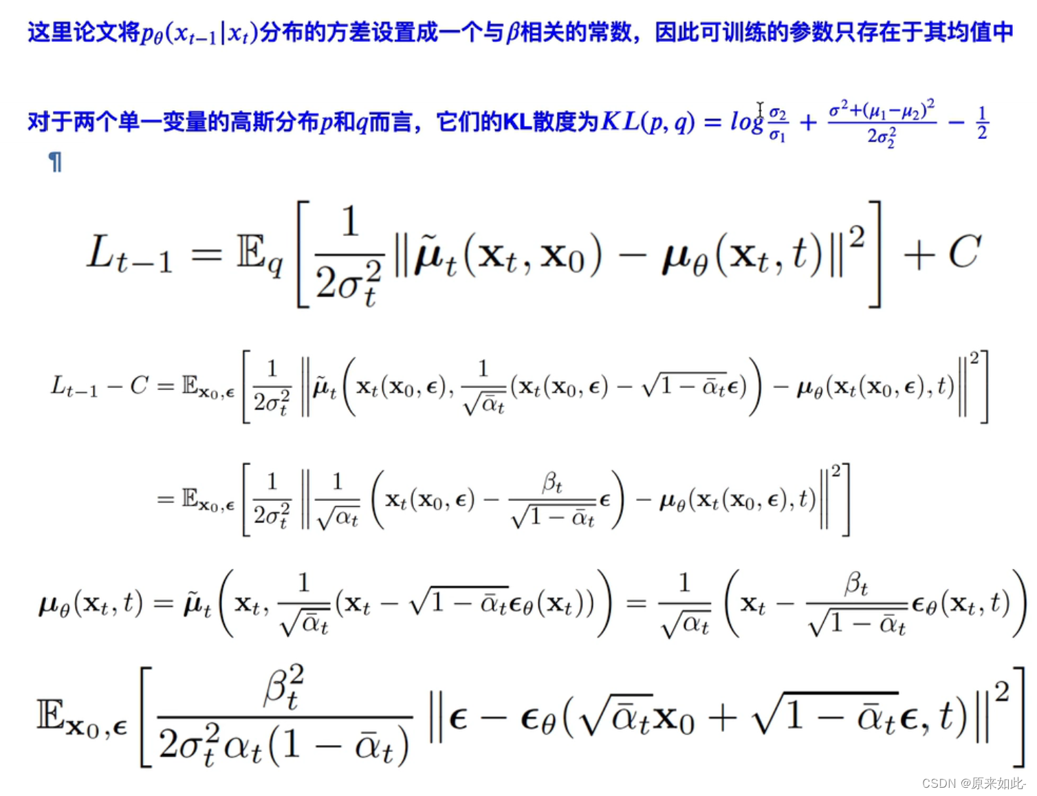
4.1 损失函数公式推导
得到损失函数如下:

; 4.2 损失函数代码实现
def diffusion_loss_fn(model, x_0, alphas_bar_sqrt, one_minus_alphas_bar_sqrt, n_steps):
    batch_size = x_0.shape[0]

    t = torch.randint(0, n_steps, size=(batch_size//2,))

    t = torch.cat([t, num_steps-1-t], dim=0)
    t = t.unsqueeze(-1)

    a = alphas_bar_sqrt[t].to(device)

    aml = one_minus_alphas_bar_sqrt[t].to(device)

    e = torch.randn_like(x_0).to(device)

    x = x_0 * a + e * aml

    output = model(x, t.squeeze(-1).to(device))

    return (e - output).square().mean()
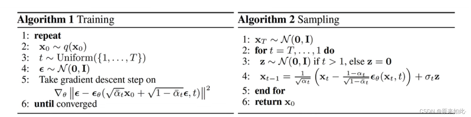
五、算法流程
; 5.1 模型训练代码
print('训练模型...')

batch_size = 128
dataloader = torch.utils.data.DataLoader(dataset, batch_size=batch_size, shuffle=True)
num_epoch = 4000
plt.rc('text', color='blue')

model = MLPDiffusion(num_steps)
model = model.to(device)
optimizer = torch.optim.Adam(model.parameters(), lr=1e-3)

for t in range(num_epoch):
    for idx, batch_x in enumerate(dataloader):
        batch_x = batch_x.to(device)
        loss = diffusion_loss_fn(model,batch_x,alphas_bar_sqrt,one_minus_alphas_bar_sqrt,num_steps)
        optimizer.zero_grad()
        loss.backward()
        torch.nn.utils.clip_grad_norm_(model.parameters(), 1.)
        optimizer.step()

    if(t%100==0):
        print(loss)
torch.save(model, "model.h5")
5.2 模型采样代码
def p_sample_loop(model, shape, n_steps, betas, one_minus_alphas_bar_sqrt):
    cur_x = torch.randn(shape).to(device)
    x_seq = [cur_x]
    for i in reversed(range(n_steps)):
        cur_x = p_sample(model, cur_x, i, betas.to(device), one_minus_alphas_bar_sqrt.to(device))
        x_seq.append(cur_x)
    return x_seq

def p_sample(model, x, t, betas, one_minus_alphas_bar_sqrt):
    t = torch.tensor([t]).to(device)
    coeff = betas[t]/one_minus_alphas_bar_sqrt[t]
    eps_theta = model(x, t)

    mean = (1 / (1-betas[t]).sqrt())*(x - (coeff*eps_theta))
    z = torch.randn_like(x).to(device)

    sigma_t = betas[t].sqrt().to(device)
    sample = mean + sigma_t * z
    return (sample)

model = torch.load("model.h5")
x_seq = p_sample_loop(model, dataset.shape, num_steps, betas, one_minus_alphas_bar_sqrt)
fig, axs = plt.subplots(1, 10, figsize=(28, 3))
for i in range(1, 11):
    cur_x = x_seq[i*10].detach()
    axs[i-1].scatter(cur_x[:, 0].cpu(), cur_x[:, 1].cpu(), color='red', edgecolor='white');
    axs[i-1].set_axis_off();
    axs[i-1].set_title('$q(\mathbf{x}_{'+str(i*10)+'})$')
5.3 训练好的模型效果

Original: https://blog.csdn.net/sunningzhzh/article/details/125118688
Author: 原来如此-
Title: Diffusion model—扩散模型
原创文章受到原创版权保护。转载请注明出处:https://www.johngo689.com/605403/
转载文章受原作者版权保护。转载请注明原作者出处!