logistic回归篇章

数据集接应上一节数据集合，本次的分析是从用户是否为高响应用户进行划分，使用logistic回归对用户进行响应度预测，得到响应的概率。线性回归，参考上一篇章

1 读取和预览数据

对数据进行加载读取，数据依旧是脱敏数据，

file_path<-"data_response_model.csv" #change the location # read in data options(stringsasfactors="F)" raw<-read.csv(file_path) #read your csv str(raw) #check varibale type view(raw) #take a quick look at summary(raw) summary of variable response view(table(raw$dv_response)) #y view(prop.table(table(raw$dv_response))) frequency < code></-"data_response_model.csv">

根据业务确定，数据的y值是响应率是dv_response，并观察其情况

2 划分数据

依旧把数据划分为三部分，分别为训练集，验证集和测试集。

#Separate Build Sample
train<-raw[raw$segment=='build',] #select build sample, it should be random selected when you the model view(table(train$segment)) #check segment view(table(train$dv_response)) y distribution view(prop.table(table(train$dv_response))) #separate invalidation sample test<-raw[raw$segment="='inval',]" invalidation(oos) view(table(test$segment)) view(prop.table(table(test$dv_response))) out of validation validation<-raw[raw$segment="='outval',]" validation(oot) view(table(validation$segment)) view(prop.table(table(validation$dv_response))) < code></-raw[raw$segment=='build',]>

3 profilng制作

对数据即中的响应率进行求和，原数据中高响应客户为1，低响应客户为0.求和的总数就是高响应客户数，length就是总记录数，求出其平均数即为总体平均数

overall performance
overall_cnt=nrow(train)   #calculate the total count
overall_resp=sum(train$dv_response)  #calculate the total responders count
overall_resp_rate=overall_resp/overall_cnt  #calculate the response rate
overall_perf<-c(overall_count=overall_cnt,overall_responders=overall_resp,overall_response_rate=overall_resp_rate) #combine overall_perf<-c(overall_cnt="nrow(train),overall_resp=sum(train$dv_response),overall_resp_rate=sum(train$dv_response)/nrow(train))" view(t(overall_perf)) #take a look at the summary < code></-c(overall_count=overall_cnt,overall_responders=overall_resp,overall_response_rate=overall_resp_rate)>

这里做的划分如同上一章节的划分lift图制作，也可用sql语句来写，如同group by，计算出每组的平均响应率与总体响应率的比较。
在library之前，请先下载plyr包，写sql需下载sqldf
install.packages(“sqldf”)

library(plyr)              #call plyr
?ddply
prof<-ddply(train,.(hh_gender_m_flag),summarise,cnt=length(rid),res=sum(dv_response)) #group by hh_gender_m_flg view(prof) #check the result tt="aggregate(train[,c("hh_gender_m_flag","rid")],by=list(train[,c("hh_gender_m_flag")]),length)" view(tt) #calculate probablity #prop.table(as.matrix(prof[,-1]),2) #t(t(prof) colsums(prof)) prof1<-within(prof,{res_rate<-res cnt index<-res_rate overall_resp_rate*100 percent<-cnt overall_cnt }) #add response_rate,index, percentage view(prof1) < code></-ddply(train,.(hh_gender_m_flag),summarise,cnt=length(rid),res=sum(dv_response))>

library(sqldf)

整型乘浮点型变浮点数据

sqldf(“select hh_gender_m_flag,count(_) as cnt,sum(dv_response)as res,1.0_sum(dv_response) /count(*) as res_rate from train group by 1 “)
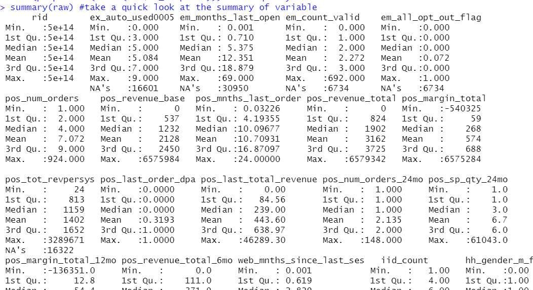
缺失值也能作为特征的一部分，同样可以对缺失值进行lift比较

nomissing<-data.frame(var_data[!is.na(var_data$em_months_last_open),]) #select the no missing value records missing<-data.frame(var_data[is.na(var_data$em_months_last_open),]) ###################################### numeric profiling:missing part ############################################################# missing2<-ddply(missing,.(em_months_last_open),summarise,cnt="length(dv_response),res=sum(dv_response))" #group by em_months_last_open view(missing2) missing_perf<-within(missing2,{res_rate<-res cnt index<-res_rate overall_resp_rate*100 percent<-cnt overall_cnt var_category<-c('unknown') }) #summary view(missing_perf) < code></-data.frame(var_data[!is.na(var_data$em_months_last_open),])>

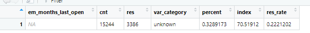
这里对非缺失值数据进行了划分，将非缺失值数据，按照十分位数划分成了10等分。分别计算其总记录数和总高响应客户数量

nomissing_value<-nomissing$em_months_last_open 10 #put the nomissing values into a variable #method1:equal frequency nomissing$var_category<-cut(nomissing_value,unique(quantile(nomissing_value,(0:10) 10)),include.lowest="T)#separte" groups based on records class(nomissing$var_category) view(table(nomissing$var_category)) #take look at category prof2<-ddply(nomissing,.(var_category),summarise,cnt="length(dv_response),res=sum(dv_response))" #group by view(prof2) < code></-nomissing$em_months_last_open>

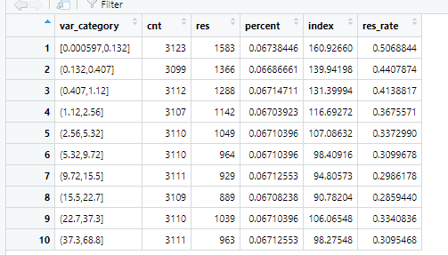
再次对划分为10等分的数据每一组都进行lift计算，比较每组的平均高响应用户数与总体的用户数的比值。大于100%就是高于总体表现的客户标签

nonmissing_perf<-within(prof2, 2 {res_rate<-res cnt index<-res_rate overall_resp_rate*100 percent<-cnt overall_cnt }) #add resp_rate,index,percent view(nonmissing_perf) #set missing_perf and non-missing_perf together view(missing_perf) em_months_last_open_perf<-rbind(nonmissing_perf,missing_perf[,-1]) data view(em_months_last_open_perf) < code></-within(prof2,>

4 缺失值，异常值处理

1 少于3%直接删除或者中位数，平均数填补
2 3%——20%删除或knn，EM回归填补
3 20%——50% 多重插补
4 50——80%缺失值分类法
5 高于80%丢弃，数据太不准确了，分析失误性很大

异常值通常用盖帽法解决

numeric variables

train$m2_em_count_valid <- 1 2 ifelse(is.na(train$em_count_valid)="=" t, 2, #when em_count_valid is missing ,then assign ifelse(train$em_count_valid <="1," 1, em_count_valid<="1" then>=10, 10, #when em_count_valid>=10 then assign 10
                                                train$em_count_valid)))        #when 1<em_count_valid<10 and not missing then assign the raw value summary(train$m2_em_count_valid) #do a summary summary(train$m1_em_count_valid) < code></em_count_valid<10></->

5 模型拟合

根据业务选取最有价值的变量

library(picante)  #call picante
var_list<-c('dv_response','m1_pos_num_orders_24mo', 'm1_pos_num_orders', 'm1_sh_mnths_last_inquired', 'm1_pos_sp_qty_24mo', 'm1_pos_revenue_total', 'm1_pos_last_order_dpa', 'm1_pos_margin_total', 'm1_pos_mo_btwn_fst_lst_order', 'm1_pos_revenue_base', 'm1_pos_tot_revpersys', 'm1_em_count_valid', 'm1_em_num_open_30', 'm1_pos_margin_total_12mo', 'm1_ex_auto_used0005_x5', 'm1_sh_inquired_last3mo', 'm1_ex_auto_used0005_x789', 'm1_hh_income', 'm1_sh_inquired_last12mo', 'm1_pos_last_total_revenue', 'm1_em_all_opt_out_flag', 'm1_pos_revenue_total_6mo', 'm1_em_months_last_open', 'm1_pos_mnths_last_order', 'm1_web_mnths_since_last_ses') #put the variables you want to do correlation analysis here < code></-c('dv_response','m1_pos_num_orders_24mo',>

制作相关系数矩阵，根据相关性筛选变量相关的，共线性选择标识变量法或哑变量法，logistic回归可使用IV值选择变量

corr_var<-train[, var_list] #select all the variables you want to do correlation analysis str(corr_var) #check variable type correlation<-data.frame(cor.table(corr_var,cor.method="pearson" )) #do view(correlation) cor_only="data.frame(row.names(correlation),correlation[," 1:ncol(corr_var)]) result only view(cor_only) < code></-train[,>

选择完，准备放到模型里面的变量

var_list<-c('m1_web_mnths_since_last_ses', 'm1_pos_mnths_last_order', 'm1_pos_num_orders_24mo', 'm1_pos_mo_btwn_fst_lst_order', 'm1_em_count_valid', 'm1_pos_tot_revpersys', 'm1_em_months_last_open', 'm1_pos_last_order_dpa' ) #put the variables you want to try in model here < code></-c('m1_web_mnths_since_last_ses',>

mods

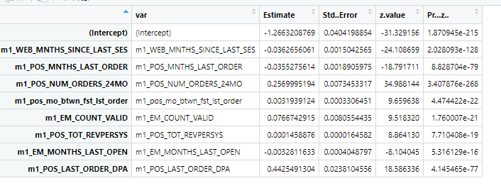
mods<-train[,c('dv_response',var_list)] #select y and varibales you want to try str(mods) (model_glm<-glm(dv_response~.,data="mods,family" =binomial(link="logit" ))) #logistic model model_glm #stepwise library(mass) model_sel<-stepaic(model_glm,direction="both" ) #using both backward forward stepwise selection model_sel summary<-summary(model_sel) #summary model_summary<-data.frame(var="rownames(summary$coefficients),summary$coefficients)" #do the summary view(model_summary) < code></-train[,c('dv_response',var_list)]>

对数据进行标准化后的建模，标准化的建模方便查看每个变量对y的影响程度

variable importance

standardize variable

#?scale
mods2<-scale(train[,var_list],center=t,scale=t) mods3<-data.frame(dv_response="c(train$dv_response),mods2[,var_list])" # view(mods3) (model_glm2<-glm(dv_response~.,data="mods3,family" =binomial(link="logit" ))) #logistic model (summary2<-summary(model_glm2)) model_summary2<-data.frame(var="rownames(summary2$coefficients),summary2$coefficients)" #do the summary view(model_summary2) model_summary2_f<-model_summary2[model_summary2$var!="(Intercept)" ,] model_summary2_f$contribution<-abs(model_summary2_f$estimate) (sum(abs(model_summary2_f$estimate))) view(model_summary2_f) < code></-scale(train[,var_list],center=t,scale=t)>

6 模型评估

回归拟合的VIF值

#Variable VIF
fit <- lm(dv_response~., data="mods)" #regression model #install.packages('car') #install package 'car' to calculate vif require(car) #call car #get var_vif="data.frame(var=rownames(vif),vif)" variables and corresponding view(var_vif) < code></->

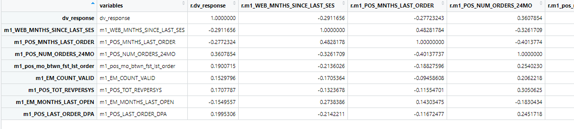
相关系数矩阵制作

#variable correlation
cor<-data.frame(cor.table(mods,cor.method = 'pearson')) #calculate the correlation correlation<-data.frame(variables="rownames(cor),cor[," 1:ncol(mods)]) #get only view(correlation) < code></-data.frame(cor.table(mods,cor.method>

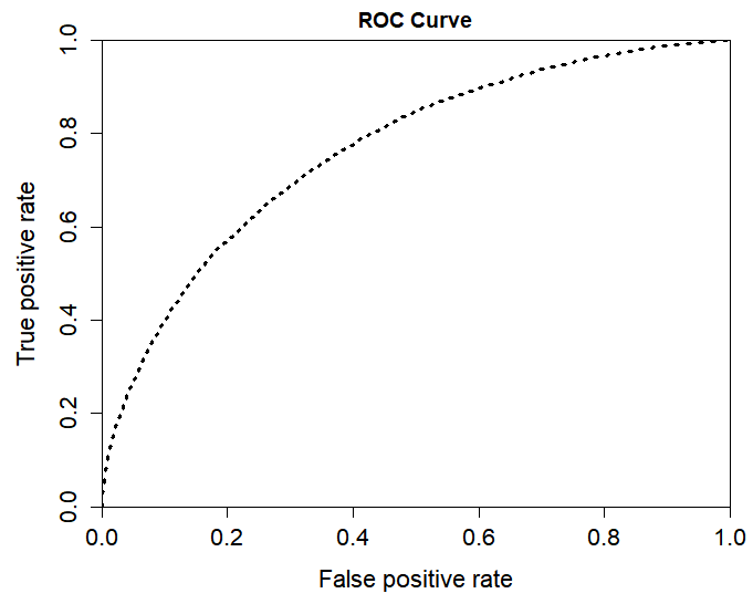
最后制作ROC曲线，对模型画ROC曲线图，观察其效果

library(ROCR)

#### test data####
pred_prob<-predict(model_glm,test,type='response') #predict y pred_prob pred<-prediction(pred_prob,test$dv_response) #put predicted and actual together pred@predictions view(pred) perf<-performance(pred,'tpr','fpr') #check the performance,true positive rate perf par(mar="c(5,5,2,2),xaxs" = "i",yaxs="i" ,cex.axis="1.3,cex.lab=1.4)" #set graph parameter #auc value auc <- performance(pred,"auc") unlist(slot(auc,"y.values")) #plotting roc curve plot(perf,col="black" ,lty="3," lwd="3,main='ROC" curve') < code></-predict(model_glm,test,type='response')>

plot Lift chart

perf

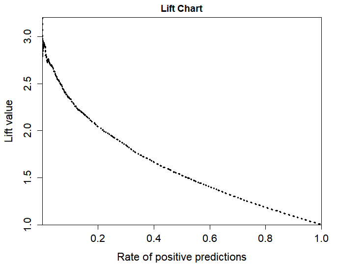
7 总体划分用户群lift图

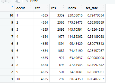
pred<-predict(model_glm,train,type='response') 10 #predict y decile<-cut(pred,unique(quantile(pred,(0:10) 10)),labels="10:1," include.lowest="T)" #separate into groups sum<-data.frame(actual="train$dv_response,pred=pred,decile=decile)" #put actual y,predicted y,decile together decile_sum<-ddply(sum,.(decile),summarise,cnt="length(actual),res=sum(actual))" #group by decile decile_sum2<-within(decile_sum, {res_rate<-res cnt index<-100*res_rate (sum(res) sum(cnt)) }) #add resp_rate,index decile_sum3<-decile_sum2[order(decile_sum2[,1],decreasing="T),]" #order view(decile_sum3) < code></-predict(model_glm,train,type='response')>

采用的是十分位数划分，等记录数的划分客户群体，可以发现1-10个层次的用户，真实响应率lift值不错。
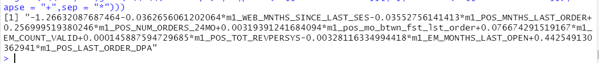
将回归方程贴出来

ss <- summary(model_glm) #put model summary together ss which(names(ss)="="coefficients")" #xbeta #y="1/(1+exp(-XBeta))" #output equoation gsub("\\+-","-",gsub('\\*\\(intercept)','',paste(ss[["coefficients"]][,1],rownames(ss[["coefficients"]]),collapse="+" ,sep="*" ))) < code></->

Original: https://blog.csdn.net/weixin_44498127/article/details/124353690
Author: THE ORDER
Title: 89 logistic回归用户画像用户响应度预测2