

文章目录
- 摘要
- 一. 条件GAN以及最小二乘GAN的原理与代码实现
* - 1.1 CGAN与原始GAN的不同与优势
- 1.2 CGAN的代码实现
- 1.3 LSCGAN的原理
– - 1.4 LSCGAN的改进代码实现
- 二. 从代码出发看懂Informer 模型并复现
* - 2.1 模型的Encoder与Dencoder得输入到底是什么样的?
– - 时序数据是如何扔给informer的
- 2.2 Embedding分析
– - 2.3 Encoder编码器
- 三. 总结
摘要
Understanding the core idea of the original GAN model and the reproduction of the code, and discovering the defects and deficiencies of GAN, and learning the CGAN principle and simple accomplished of the GAN code in this article, the CGAN model is realized; and the principle interpretation of the LSGAN model , and discussed that the original GAN used the cross-entropy loss function and replaced it with the least squares loss function, which improved two problems of the traditional GAN. On the basis of the CGAN code, the code reproduction of the LSCGAN model is realized, but it is based on the simplest internal DNN structure network, and does not use a more complex network.
Informer model From the perspective of code, we re-understand how its time series data is thrown to the informer, what is the input of the model’s Encoder and Decoder, how the data is read, the construction of dataloader and dataset, etc.; And the most innovative implementation code of the unified embedding of timestamp encoding, data encoding and absolute position encoding; the implementation of Encoder encoder, the most innovative point is the sparse attention mechanism and distillation operation, the code implementation process is also more complex.
对原始GAN模型的核心思想理解与代码的复现,与发现GAN的缺陷与不足,并学习了本篇中的CGAN原理与简单改造GAN代码,便实现了CGAN模型;还有LSGAN模型的原理解读,与论述了原始GAN采用的是交叉熵损失函数,并将其替换成最小二乘损失函数,这改善了传统 GAN 的两个问题。也在CGAN代码的基础上,实现了LSCGAN模型的代码复现,但它是基于最简单的内部是DNN结构的网络,并没有采用更为复杂的网络。
Informer模型我们从代码的角度出发,重新理解其时序数据是如何扔给informer的,以及模型的Encoder与Dencoder得输入到底是什么样的,数据是怎样读取的,dataloader与dataset的构建等等;以及最具创新的时间戳编码与数据编码与绝对位置编码的统一embedding 的实现代码;Encoder编码器的实现,其中最为创新点就是稀疏注意力机制与蒸馏操作,其代码实现过程也是较为复杂的。
一. 条件GAN以及最小二乘GAN的原理与代码实现
1.1 CGAN与原始GAN的不同与优势
CGAN论文的下载地址: CGAN下载论文
GAN的核心思想是:同时训练两个相互协作、同时又相互竞争的深度神经网络。一个称为生成器Generator,另一个称为判别器Discriminator)来处理 无监督学习的相关问题。
传统GAN 的优化目标:

回顾GAN的训练目的:
- 生成模型G构建一个从先验分布Pz (z)到数据空间的映射函数 G(z; θg)。判别模型D的输入是真实图像或者生成图像,D(x; θd )输出一个标量, 表示输入样本来自训练样本(而非生成样本)的概率;
- 模型G和D同时训练: 1、固定判别模型D,训练生成器G,调整G的参数使得log(1 – D((G))的期望最小化;实际就是让D(G(z))的期望最大化,接近于1;
- 固定生成模型G,训练判别器D,调整D的参数使得logD(X) + log(1 – D(G(z))的期望最大化。
GAN的缺陷:
从训练过程来看,基于手写数字识别的样本中,从判别器看,无论是真实的 x x x,还是预测的样本G ( z ) G(z)G (z ),它的输入都只有一个,但在数据集中有十类(0-9),没有给生成器任何的当前信息,这个任务会加大GAN的训练难度!所以便 引入C这一个条件变量,比如标签y,作为条件信息,将其作为G与D的输入!
CAGAN的不同之处:
条件生成式对抗网络(CGAN) 是对原始GAN的一个扩展,生成器和判别器都增加额外信息 y为条件, y可以使任意信息,例如类别信息, 标签信息,或者其他模态的数据。通过将额外信息y输送给判别模型和生成模型, 作为输入层的一部分,从而实现条件GAN。


如何将标签y 信息加入到G与D的输入中,一般是采用embedding cat起来的做法,就如上图展示的一样。
在生成模型中,先验输入噪声p(z)和条件信息y联合组成了联合隐层表征。条件GAN的目标函数是带有条件概率的二人极小极大值博弈(two-player minimax game ) ,如果 条件变量y是类别标签,可以看做CGAN是把纯无监督的GAN变成有监督的模型的一种改进。
; 1.2 CGAN的代码实现
我们还是基于上次实现过的原始GAN的那个例子上继续改进即可,主要就是对输入进行修改,需要 添加 label_embedding操作。
改进点1:生成器中
class Generator(nn.Module):

    def __init__(self):
        super(Generator, self).__init__()
        self.embedding = nn.Embedding(10,label_emb_dim)

        self.model = nn.Sequential(
            nn.Linear(latent_dim+label_emb_dim, 128),
            torch.nn.BatchNorm1d(128),
            torch.nn.ReLU(inplace = True),

            nn.Linear(128, 256),
            torch.nn.BatchNorm1d(256),
            torch.nn.ReLU(inplace=True),
            nn.Linear(256, 512),
            torch.nn.BatchNorm1d(512),
            torch.nn.ReLU(inplace=True),
            nn.Linear(512, 1024),
            torch.nn.BatchNorm1d(1024),
            torch.nn.ReLU(inplace=True),
            nn.Linear(1024, np.prod(image_size, dtype=np.int32)), # np.prod()连乘操作
            #  nn.Tanh(),
            nn.Sigmoid(),
        )

    def forward(self, z,labels):
        # shape of z: [batchsize, latent_dim]

        # 在生成器中引入条件信息
        labels_embedding = self.embedding(labels)
        z = torch.cat([z,labels_embedding],axis= -1)

        output = self.model(z)
        image = output.reshape(z.shape[0], *image_size)
        return image
改进点2:判别器中也只是做了一点点调整
class Discriminator(nn.Module):

    def __init__(self):
        super(Discriminator, self).__init__()
        self.embedding = nn.Embedding(10, label_emb_dim)

        self.model = nn.Sequential(
            nn.Linear(np.prod(image_size, dtype=np.int32)+label_emb_dim, 512),
            torch.nn.ReLU(),
            nn.Linear(512, 256),
            torch.nn.GELU(),
            nn.Linear(256, 128),
            torch.nn.ReLU(),
            nn.Linear(128, 64),
            torch.nn.ReLU(),
            nn.Linear(64, 32),
            torch.nn.ReLU(),
            nn.Linear(32, 1),
            nn.Sigmoid(),
        )

    def forward(self, image,labels):
        # shape of image: [batchsize, 1, 28, 28]
        labels_embedding = self.embedding(labels)
        prob = self.model(torch.cat([image.reshape(image.shape[0], -1),labels_embedding],axis=-1)) # 将四维的变成二维的,送入判别器model,得出一个概率

        return prob
改进点3:
#从mini_batch中获取labels
 gt_images, labels = mini_batch   # mini_batch包含 x和y,label这里就也需要了(当成条件)

把Z,与labels 都 喂入生成器中,得出预测的images照片
pred_images = generator(z,labels)
改进点4:
#还有就是对G与D进行优化的loss 中都必须引入labels
对生成器进行优化
        # discriminator(pred_images)是判别器对预测图片给出的概率大小,labels_one则是target,对生成器G进行优化,target取1;
        g_loss = recons_loss*0.05 + loss_fn(discriminator(pred_images,labels), labels_one
        )
#判别器的目标函数有两项
        real_loss = loss_fn(discriminator(gt_images,labels), labels_one) # 对真实图片预测成 1
        fake_loss = loss_fn(discriminator(pred_images.detach(),labels), labels_zero)
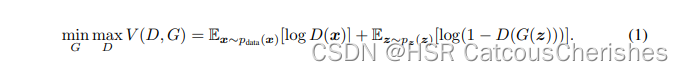
下面展示CGAN的执行效果与GAN的同一步骤下的对比:
GAN——image_4548.png
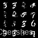
CGAN——image_C4548.png
从上图中确实可以看出CGAN的效果要比GAN好一些的!
1.3 LSCGAN的原理
1.3.1 与GAN的最大区别
参考原始论文地址: LSGAN
传统 GAN 生成的图片质量不高,这是由于GAN使用的是交叉熵损失(sigmoid cross entropy)作为判别器D的损失函数。这种损失函数在学习过程中会导致梯度消失的问题,使其很难再去更新生成器。为克服这一点,提出LSGAN模型,LSGANs 这篇经典的论文主要工作是把GAN中 交叉熵损失函数替换成最小二乘损失函数,这改善了传统 GAN 的两个问题,即传统 GAN 生成的图片质量不高,而且训练过程十分不稳定。
我们知道 交叉熵一般都是拿来做逻辑分类的,而像 最小二乘这种一般会用 在线性回归中,这里用最小二乘作为损失函数的评判!
1.3.2 method对比
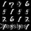
先回顾什么是梯度消失现象,这里利用一个简单的例子画出饱和图形:饱和的意思就是梯度一直处于0的位置,不利于更新。
nn.BCELoss  Examples:
#
>>> m = nn.Sigmoid()
>>> loss = nn.BCELoss()
>>> input = torch.randn(3, requires_grad=True)
>>> target = torch.empty(3).random_(2)
>>> output = loss(m(input), target)
>>> output.backward()

import torch
import torch.nn as nn
import matplotlib.pyplot as plt

logits = torch.linspace(-10,10,2000)
loss=[]
loss_fn = nn.BCELoss()
m=nn.Sigmoid()

for lgs in logits:
    loss_1=loss_fn(m(lgs), torch.ones_like(lgs))

    loss.append(loss_1)

plt.plot(logits,loss)
plt.show()
LSGAN的目标优化函数:
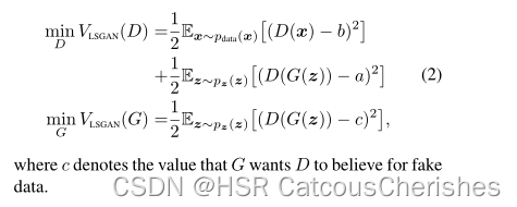
其中 G 为生成器(Generator),D 为判别器(Discriminator),z 为噪音,它可以服从归一化或者高斯分布,P d a t a ( x ) P_{data}(x)P d a t a (x )为真实数据 x 服从的概率分布, P z ( z ) P_{z}(z)P z (z )为 z 服从的概率分布。 E x − P d a t a ( x ) E_{x-P_{data}(x)}E x −P d a t a (x ) 为期望值,E z − P z ( z ) E_{z-P_{z}(z)}E z −P z (z ) 同为期望值。
作者提出了两种 abc 的取值方法:其推导过程较为复杂,原文中有
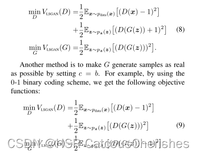
下面采用公式9去作LSGAN目标优化函数。
当优化判别器D时,对于真实样本x设置目标值是1,对虚假样本设置成0;当优化生成器G时,将生成的样本标签也设置为1。
1.4 LSCGAN的改进代码实现
本次只是在CGAN的基础上,将交叉熵损失函数替换成最小二乘损失函数,其他的G与D内部的模型,依然是采用的DNN,所以该效果区别不是很大,要想效果更好,需要去作模型内部框架的升级才行了!
BCELoss()损失函数,二项的交叉熵函数,定义部分
#loss_fn = nn.BCELoss()
将分类任务变成一个回归任务
loss_fn = nn.MSELoss()
二. 从代码出发看懂Informer 模型并复现
参考博客列表:
1. 细读informe模型
2.AAAI2021最佳论文-informer[1] 主要思想和代码
3.AAAI最佳论文Informer 解读
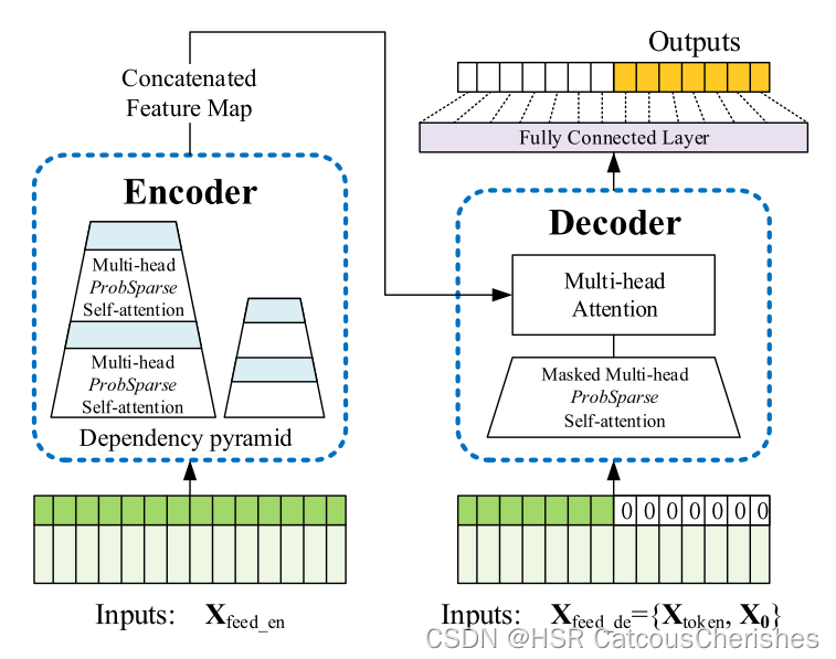
; 2.1 模型的Encoder与Dencoder得输入到底是什么样的?
数据介绍:ETDataset(Electricity Transformer Dataset)电力变压器的负荷、油温数据。论文作者给出的数据下载地址:ETDataset(github)
我们举一个 例子,看懂inforemr模型得输入:
2.1 1. Encoder输入
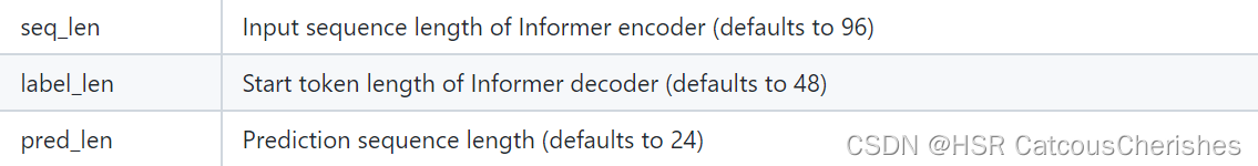
首先认清这三个 超参数hyperparameter:
date=2016-07-01 00:00 是一个时间点0的数据
date=2016-07-01 01:00 是时间点1的数据。
那么滑动序列窗口长为96:
即批次中的样本1:时间点0到时间点95的96个维度为7的数据
批次中的样本2:时间点1到时间点96的96个维度为7的数据
批次中的样本3:时间点2到时间点97的96个维度为7的数据
……
直到取够32个样本,形成一个批次内的所有样本。
与其他模型不同的输入点:在于对 时间戳的处理上。将date列的内容编码为时间戳,主要是通过utils中的timeFeatures.py文件实现,主要是进行以下的转换(以freq=’h’为例),转化后的4维变量每一维分别代表【月份、日期、星期、小时】:
代码中utils中的timeFeatures.py文件内的time_features函数,该函数的实现如下
def time_features(dates, timeenc=1, freq='h'):
"""
    > time_features takes in a dates dataframe with a 'dates' column and extracts the date down to freq where freq can be any of the following if timeenc is 0:
    > * m - [month]
    > * w - [month]
    > * d - [month, day, weekday]
    > * b - [month, day, weekday]
    > * h - [month, day, weekday, hour]
    > * t - [month, day, weekday, hour, *minute]
    >
    > If timeenc is 1, a similar, but different list of freq values are supported (all encoded between [-0.5 and 0.5]):
    > * Q - [month]
    > * M - [month]
    > * W - [Day of month, week of year]
    > * D - [Day of week, day of month, day of year]
    > * B - [Day of week, day of month, day of year]
    > * H - [Hour of day, day of week, day of month, day of year]
    > * T - [Minute of hour*, hour of day, day of week, day of month, day of year]
    > * S - [Second of minute, minute of hour, hour of day, day of week, day of month, day of year]

    *minute returns a number from 0-3 corresponding to the 15 minute period it falls into.

"""
    # timeenc = 0 if args.embed!='timeF' else 1
    if timeenc==0:
        dates['month'] = dates.date.apply(lambda row:row.month,1)
        dates['day'] = dates.date.apply(lambda row:row.day,1)
        dates['weekday'] = dates.date.apply(lambda row:row.weekday(),1)
        dates['hour'] = dates.date.apply(lambda row:row.hour,1)
        dates['minute'] = dates.date.apply(lambda row:row.minute,1)
        dates['minute'] = dates.minute.map(lambda x:x
        freq_map = {
            'y':[],'m':['month'],'w':['month'],'d':['month','day','weekday'],
            'b':['month','day','weekday'],'h':['month','day','weekday','hour'],
            't':['month','day','weekday','hour','minute'],
        }
        return dates[freq_map[freq.lower()]].values
    if timeenc==1:
        dates = pd.to_datetime(dates.date.values)
        # time_features_from_frequency_str返回的是对应freq下的时间归一化对象列表,处理后会将时间按照需要的格式归一化到-0.5到0.5之间
        return np.vstack([feat(dates) for feat in time_features_from_frequency_str(freq)]).transpose(1,0)
得出时间戳 X m a r k X_{mark}X m a r k : 32×96×4;
4代表 时间戳,例如我们用小时维度的数据,那么4分别代表 年、月、日、小时;
第一个时间点对应的时间戳就是[2016, 07, 01, 00],
第二个时间点对应的时间戳就是[2016, 07, 01, 01]
与上面的 X e n c X_{enc}X e n c 对应得到所有的样本对应的时间戳。
2.1.2 Decoder输入
decoder的输入与encoder唯一不同的就是,每个样本对应时间序列的时间点数量并不是96,而是72。具体在进行截取样本时,从encoder输入的后半段开始取。
X d e c X_{dec}X d e c =(X s t o k e , 0 ) X_{stoke},0)X s t o k e ,0 )=32 ∗ ( 48 + 24 ) ∗ 7 32(48+24)7 3 2 ∗(4 8 +2 4 )∗7
即:encoder的第一个样本:时间点0到时间点95的96条维度为7的数据
那与之对应decoder的:时间点47到时间点95的48条维度为7的数据 (取后一半48条数据——label_seq=48)+ 时间点 95到时间点119的24个时间点(pred_seq=24)的7维数据;则最终48+24是72维度的数据。
同样的加入时间戳维度输入: X m a r k X_{mark}X m a r k :32 × 72 × 4 32×72×4 3 2 ×7 2 ×4
时序数据是如何扔给informer的
这里部分便是代码data_loader.py中Dataset_ETT_hour等的构建,以及__read_data__函数与 __getitem__函数是如何实现的。
以 Dataset_ETT_hour的构建划分为例子,数据是ETTh1.csv:
class Dataset_ETT_hour(Dataset):
    def __init__(self, root_path, flag='train', size=None,
                 features='S', data_path='ETTh1.csv',
                 target='OT', scale=True, inverse=False, timeenc=0, freq='h', cols=None):
        # size [seq_len, label_len, pred_len]
        # info
        if size == None:
            self.seq_len = 24*4*4
            self.label_len = 24*4
            self.pred_len = 24*4
        else:
            self.seq_len = size[0]
            self.label_len = size[1]
            self.pred_len = size[2]
        # init
        assert flag in ['train', 'test', 'val']
        type_map = {'train':0, 'val':1, 'test':2}
        self.set_type = type_map[flag]

        self.features = features
        self.target = target
        self.scale = scale
        self.inverse = inverse
        self.timeenc = timeenc
        self.freq = freq

        self.root_path = root_path
        self.data_path = data_path
        self.__read_data__()

    def __read_data__(self):
        self.scaler = StandardScaler()
        df_raw = pd.read_csv(os.path.join(self.root_path,
                                          self.data_path))

        border1s = [0, 12*30*24 - self.seq_len, 12*30*24+4*30*24 - self.seq_len]
        border2s = [12*30*24, 12*30*24+4*30*24, 12*30*24+8*30*24]
        border1 = border1s[self.set_type]
        border2 = border2s[self.set_type]

        if self.features=='M' or self.features=='MS':
            cols_data = df_raw.columns[1:]
            df_data = df_raw[cols_data]
        elif self.features=='S':
            df_data = df_raw[[self.target]]

        if self.scale:
            train_data = df_data[border1s[0]:border2s[0]]
            self.scaler.fit(train_data.values)
            data = self.scaler.transform(df_data.values)
        else:
            data = df_data.values

        df_stamp = df_raw[['date']][border1:border2]
        df_stamp['date'] = pd.to_datetime(df_stamp.date)
        data_stamp = time_features(df_stamp, timeenc=self.timeenc, freq=self.freq)

        self.data_x = data[border1:border2]
        if self.inverse:
            self.data_y = df_data.values[border1:border2]
        else:
            self.data_y = data[border1:border2]
        self.data_stamp = data_stamp

    def __getitem__(self, index):
        s_begin = index
        s_end = s_begin + self.seq_len
        r_begin = s_end - self.label_len
        r_end = r_begin + self.label_len + self.pred_len

        seq_x = self.data_x[s_begin:s_end]
        if self.inverse:
            seq_y = np.concatenate([self.data_x[r_begin:r_begin+self.label_len], self.data_y[r_begin+self.label_len:r_end]], 0)
        else:
            seq_y = self.data_y[r_begin:r_end]
        seq_x_mark = self.data_stamp[s_begin:s_end]
        seq_y_mark = self.data_stamp[r_begin:r_end]

        return seq_x, seq_y, seq_x_mark, seq_y_mark

    def __len__(self):
        return len(self.data_x) - self.seq_len- self.pred_len + 1

    def inverse_transform(self, data):
        return self.scaler.inverse_transform(data)
M和MS都是多变量特征标志,S是单变量特征标志。
对于数据集长度的划分:
源代码data_loader.py文件中,seq_len是Encoder输入序列的长度,label_len是Decoder中的start token的长度,输入到Encoder的seq_len长度的序列是包含label_len长度这部分序列的,pred_len是预测序列长度,所以输入到Decoder的序列长度是label_len+pred_len。
对于ETTh1这个数据集,它使用0到(12 _30_24)行作为训练集(一年的数据),(12 _30_24-seq_len)到(12 _30_24+4 _30_24)行作为测试集,(12 _30_24+4 _30_24-seq_len)到(12 _30_24+8 _30_24)作为验证集。
2.2 Embedding分析
输入:
X e n c = 32 ∗ 96 ∗ 7 X_{enc}=32967 X e n c =3 2 ∗9 6 ∗7;
Y d e c = 32 ∗ 72 ∗ 7 Y_{dec}=32727 Y d e c =3 2 ∗7 2 ∗7;
X m a r k = 32 ∗ 96 ∗ 4 X_{mark}=32964 X m a r k =3 2 ∗9 6 ∗4;
Y m a r k = 32 ∗ 72 ∗ 4 Y_{mark}=32724 Y m a r k =3 2 ∗7 2 ∗4。
输出:
embeeding 后维度
X f e n d − e n c = 32 ∗ 96 ∗ 512 X_{fend-enc}=32 * 96512 X f e n d −e n c =3 2 ∗9 6 ∗5 1 2;
X f e n d − d e = 32 ∗ 72 ∗ 512 X_{fend-de}=32 * 72512 X f e n d −d e =3 2 ∗7 2 ∗5 1 2。
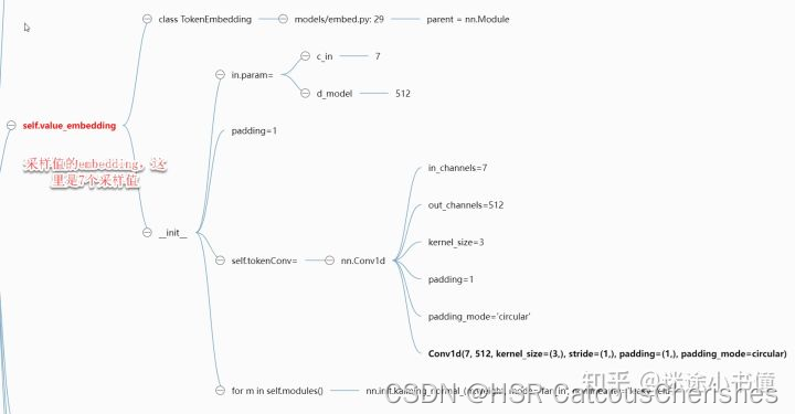
2.2.1 数据embedding—tokenEmbedding
对输入的原始数据进行一个1维卷积得到,将输入数据从C ( i n ) = 7 C(in)=7 C (i n )=7维映射为d ( m o d e l ) = 512 d(model)=512 d (m o d e l )=5 1 2 维。
实现代码如下:
class TokenEmbedding(nn.Module):
    def __init__(self, c_in, d_model):
        super(TokenEmbedding, self).__init__()
        padding = 1 if torch.__version__>='1.5.0' else 2
        # nn.Conv1d对输入序列的每一个时刻的特征进行一维卷积,且这里stride使用默认的1
        self.tokenConv = nn.Conv1d(in_channels=c_in, out_channels=d_model,
                                    kernel_size=3, padding=padding, padding_mode='circular')
        for m in self.modules():
            if isinstance(m, nn.Conv1d):
                nn.init.kaiming_normal_(m.weight,mode='fan_in',nonlinearity='leaky_relu')

    def forward(self, x):
        # https://pytorch.org/docs/master/generated/torch.nn.Conv1d.html#torch.nn.Conv1d
        # 因为Conv1d要求输入是(N, Cin, L)输出是(N, Cout, L),所以需要对输入样本维度顺序进行调整
        x = self.tokenConv(x.permute(0, 2, 1)).transpose(1,2)
        return x
主要是一个卷积网络了,从7到512映射。参考脑图来源——informer代码脑图详情1-知乎迷途
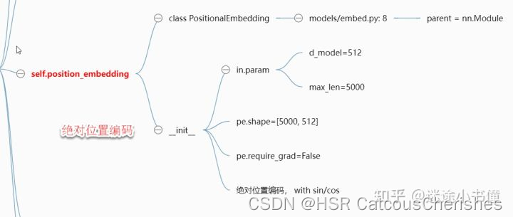
; 2.2.2 位置编码—positionEmbedding
这里的做法与transformer模型是相同的做法:都是通过sin/cos来实现位置编码区别的。
计算公式如下:
P E ( p o s , 2 i ) = s i n ( p o s / 1000 0 2 i / d m o d e l ) PE_{(pos,2i)}=sin(pos/10000^{2i/d_{model}})P E (p o s ,2 i )=s i n (p o s /1 0 0 0 0 2 i /d m o d e l )
P E ( p o s , 2 i + 1 ) = c o s ( p o s / 1000 0 2 i / d m o d e l ) PE_{(pos,2i+1)}=cos(pos/10000^{2i/d_{model}})P E (p o s ,2 i +1 )=c o s (p o s /1 0 0 0 0 2 i /d m o d e l )
源码如下:
class PositionalEmbedding(nn.Module):
    def __init__(self, d_model, max_len=5000):
        super(PositionalEmbedding, self).__init__()
        # Compute the positional encodings once in log space.

        pe = torch.zeros(max_len, d_model).float() #创建出了5000个位置的编码,但可能并不需要5000个长度的编码
        pe.require_grad = False

        position = torch.arange(0, max_len).float().unsqueeze(1) # 生成维度为[5000, 1]的位置下标向量
        div_term = (torch.arange(0, d_model, 2).float() * -(math.log(10000.0) / d_model)).exp()

        pe[:, 0::2] = torch.sin(position * div_term)
        pe[:, 1::2] = torch.cos(position * div_term)

        pe = pe.unsqueeze(0)
        self.register_buffer('pe', pe)

    def forward(self, x):
        return self.pe[:, :x.size(1)]
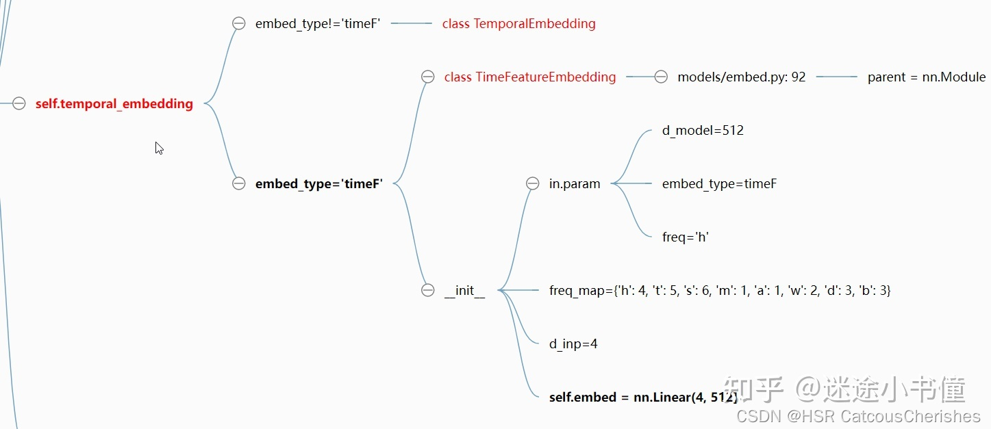
2.2.3 时间戳编码
时间戳的编码分为 TemporalEmbedding和 TimeFeatureEmbedding这两种方式,前者使用month_embed、day_embed、weekday_embed、hour_embed和minute_embed(可选)多个embedding层处理输入的时间戳,将结果相加;后者直接使用一个全连接层将输入的时间戳映射到512维的embedding。
在代码中使用区分两种方式:
if embed_type!='timeF'
下面先对方式一:TemporalEmbedding中的embedding层可以使用Pytorch自带的embedding层(nn.Embedding),再训练参数,也可以使用定义的FixedEmbedding,它使用位置编码作为embedding的参数,不需要训练参数。代码如下:
class TemporalEmbedding(nn.Module):
    def __init__(self, d_model, embed_type='fixed', freq='h'):
        super(TemporalEmbedding, self).__init__()

        minute_size = 4; hour_size = 24
        weekday_size = 7; day_size = 32; month_size = 13

        Embed = FixedEmbedding if embed_type=='fixed' else nn.Embedding
        if freq=='t':
            self.minute_embed = Embed(minute_size, d_model)
        self.hour_embed = Embed(hour_size, d_model)
        self.weekday_embed = Embed(weekday_size, d_model)
        self.day_embed = Embed(day_size, d_model)
        self.month_embed = Embed(month_size, d_model)

   def forward(self, x):
        x = x.long()
        # 在数据准备阶段,对于时间的处理时若freq='h'时'h':['month','day','weekday','hour']
        minute_x = self.minute_embed(x[:,:,4]) if hasattr(self, 'minute_embed') else 0.

        hour_x = self.hour_embed(x[:,:,3])
        weekday_x = self.weekday_embed(x[:,:,2])
        day_x = self.day_embed(x[:,:,1])
        month_x = self.month_embed(x[:,:,0])

        return hour_x + weekday_x + day_x + month_x + minute_x
class FixedEmbedding(nn.Module):
    def __init__(self, c_in, d_model):# c_in表示有多少个位置,在时间编码中表示每一维时间特征的粒度(h:24, m:4, weekday:7, day:32, month:13)
        super(FixedEmbedding, self).__init__()

        w = torch.zeros(c_in, d_model).float()
        w.require_grad = False

        position = torch.arange(0, c_in).float().unsqueeze(1)
        div_term = (torch.arange(0, d_model, 2).float() * -(math.log(10000.0) / d_model)).exp()

        w[:, 0::2] = torch.sin(position * div_term)
        w[:, 1::2] = torch.cos(position * div_term)

        self.emb = nn.Embedding(c_in, d_model)
        self.emb.weight = nn.Parameter(w, requires_grad=False)

    def forward(self, x):
        return self.emb(x).detach() #不进行训练
方式二:TimeFeatureEmbedding的实现代码如下:
class TimeFeatureEmbedding(nn.Module):
    def __init__(self, d_model, embed_type='timeF', freq='h'):
        super(TimeFeatureEmbedding, self).__init__()

        freq_map = {'h':4, 't':5, 's':6, 'm':1, 'a':1, 'w':2, 'd':3, 'b':3}
        d_inp = freq_map[freq]
        self.embed = nn.Linear(d_inp, d_model)

    def forward(self, x):
        return self.embed(x)
下面是将三者相加:三部分的embedding加起来,就得到了最终的embedding。
最终的embedding :DataEmbedding:
class DataEmbedding(nn.Module):
    def __init__(self, c_in, d_model, embed_type='fixed', freq='h', dropout=0.1):
        super(DataEmbedding, self).__init__()

        self.value_embedding = TokenEmbedding(c_in=c_in, d_model=d_model)
        self.position_embedding = PositionalEmbedding(d_model=d_model)
        #标准化后的时间才会使用TimeFeatureEmbedding,这是一个可学习的时间编码
        self.temporal_embedding = TemporalEmbedding(d_model=d_model, embed_type=embed_type, freq=freq) if embed_type!='timeF' else TimeFeatureEmbedding(d_model=d_model, embed_type=embed_type, freq=freq)

        self.dropout = nn.Dropout(p=dropout)

    #这里x的输入维度应该是[batch_size, seq_len, dim_feature],x_mark的维度应该是[batch_size, seq_len, dim_date]
    def forward(self, x, x_mark):
        # 这里将三个embedding的结果相加,具体原因可以参考
        x = self.value_embedding(x) + self.position_embedding(x) + self.temporal_embedding(x_mark)

        return self.dropout(x)
embedding部分的实现还是比较复杂的。
2.3 Encoder编码器
输入:
X f e n d − e n c = 32 ∗ 96 ∗ 512 X_{fend-enc}=32 * 96512 X f e n d −e n c =3 2 ∗9 6 ∗5 1 2;
输出:
X e n c − o u t = 32 ∗ 51 ∗ 512 X_{enc-out}=3251*512 X e n c −o u t =3 2 ∗5 1 ∗5 1 2(51应该是conv1d卷积取整导致的)
encoder部分的核心必然是计算attention。
attn.py
使用了两种attention,一种是普通的多头自注意力层(FullAttention),一种是Informer新提出来的ProbSparse self-attention层(ProbAttention)。
class FullAttention(nn.Module):
    def __init__(self, mask_flag=True, factor=5, scale=None, attention_dropout=0.1, output_attention=False):
        super(FullAttention, self).__init__()
        self.scale = scale
        self.mask_flag = mask_flag
        self.output_attention = output_attention
        self.dropout = nn.Dropout(attention_dropout)

    def forward(self, queries, keys, values, attn_mask):
        # 前向传播
        B, L, H, E = queries.shape
        _, S, _, D = values.shape
        scale = self.scale or 1./sqrt(E)

        scores = torch.einsum("blhe,bshe->bhls", queries, keys)
        if self.mask_flag:
            if attn_mask is None:
                attn_mask = TriangularCausalMask(B, L, device=queries.device)

            scores.masked_fill_(attn_mask.mask, -np.inf)

        A = self.dropout(torch.softmax(scale * scores, dim=-1))
        V = torch.einsum("bhls,bshd->blhd", A, values)

        if self.output_attention:
            return (V.contiguous(), A)
        else:
            return (V.contiguous(), None)
Informer模型中提出了一种新的注意力层——ProbSparse Self-Attention。
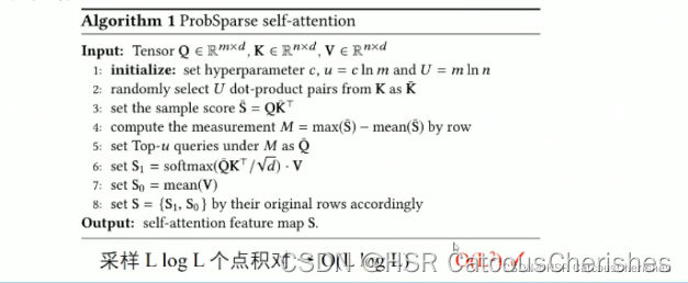
class ProbAttention(nn.Module):
    def __init__(self, mask_flag=True, factor=5, scale=None, attention_dropout=0.1, output_attention=False):
        super(ProbAttention, self).__init__()
        self.factor = factor
        self.scale = scale
        self.mask_flag = mask_flag
        self.output_attention = output_attention
        self.dropout = nn.Dropout(attention_dropout)

    def _prob_QK(self, Q, K, sample_k, n_top): # n_top: c*ln(L_q)
        # 计算QK
        # Q [B, H, L, D]
        B, H, L_K, E = K.shape
        _, _, L_Q, _ = Q.shape

        # 计算抽样的 Q_K:是否随机抽样
        K_expand = K.unsqueeze(-3).expand(B, H, L_Q, L_K, E)
        index_sample = torch.randint(L_K, (L_Q, sample_k)) # real U = U_part(factor*ln(L_k))*L_q
        K_sample = K_expand[:, :, torch.arange(L_Q).unsqueeze(1), index_sample, :]
        Q_K_sample = torch.matmul(Q.unsqueeze(-2), K_sample.transpose(-2, -1)).squeeze()

        # 使用稀疏度量查找Top_k查询
        M = Q_K_sample.max(-1)[0] - torch.div(Q_K_sample.sum(-1), L_K)
        M_top = M.topk(n_top, sorted=False)[1]

        # 使用抽样的Q来计算Q_K
        Q_reduce = Q[torch.arange(B)[:, None, None],
                     torch.arange(H)[None, :, None],
                     M_top, :] # factor*ln(L_q)
        Q_K = torch.matmul(Q_reduce, K.transpose(-2, -1)) # factor*ln(L_q)*L_k

        return Q_K, M_top

    def _get_initial_context(self, V, L_Q):
        B, H, L_V, D = V.shape
        if not self.mask_flag:
            # V_sum = V.sum(dim=-2)
            V_sum = V.mean(dim=-2)
            contex = V_sum.unsqueeze(-2).expand(B, H, L_Q, V_sum.shape[-1]).clone()
        else: # 使用掩码
            assert(L_Q == L_V) # requires that L_Q == L_V, i.e. for self-attention only (要求L_Q==L_V,即仅仅用于self-attention)
            contex = V.cumsum(dim=-2)
        return contex

    def _update_context(self, context_in, V, scores, index, L_Q, attn_mask):
        B, H, L_V, D = V.shape

        if self.mask_flag:
            attn_mask = ProbMask(B, H, L_Q, index, scores, device=V.device)
            scores.masked_fill_(attn_mask.mask, -np.inf)

        attn = torch.softmax(scores, dim=-1) # nn.Softmax(dim=-1)(scores)

        context_in[torch.arange(B)[:, None, None],
                   torch.arange(H)[None, :, None],
                   index, :] = torch.matmul(attn, V).type_as(context_in)
        if self.output_attention:
            attns = (torch.ones([B, H, L_V, L_V])/L_V).type_as(attn).to(attn.device)
            attns[torch.arange(B)[:, None, None], torch.arange(H)[None, :, None], index, :] = attn
            return (context_in, attns)
        else:
            return (context_in, None)

    def forward(self, queries, keys, values, attn_mask):
        B, L_Q, H, D = queries.shape
        _, L_K, _, _ = keys.shape

        queries = queries.transpose(2,1)
        keys = keys.transpose(2,1)
        values = values.transpose(2,1)

        U_part = self.factor * np.ceil(np.log(L_K)).astype('int').item() # c*ln(L_k)
        u = self.factor * np.ceil(np.log(L_Q)).astype('int').item() # c*ln(L_q)

        U_part = U_part if U_part<L_K else L_K
        u = u if u<L_Q else L_Q

        scores_top, index = self._prob_QK(queries, keys, sample_k=U_part, n_top=u)

        # add scale factor
        scale = self.scale or 1./sqrt(D)
        if scale is not None:
            scores_top = scores_top * scale
        # get the context
        context = self._get_initial_context(values, L_Q)
        # update the context with selected top_k queries
        context, attn = self._update_context(context, values, scores_top, index, L_Q, attn_mask)

        return context.transpose(2,1).contiguous(), attn
AttentionLayer是定义的attention层,会先将输入的embedding分别 通过线性映射得到query、key、value。还将输入维度 d m o d e l d_{model}d m o d e l 划分为多头,接着就执行前面定义的attention操作,最后经过一个线性映射得到输出。
class AttentionLayer(nn.Module):
    def __init__(self, attention, d_model, n_heads,
                 d_keys=None, d_values=None, mix=False):
        super(AttentionLayer, self).__init__()

        d_keys = d_keys or (d_model
        d_values = d_values or (d_model

        self.inner_attention = attention
        self.query_projection = nn.Linear(d_model, d_keys * n_heads)
        self.key_projection = nn.Linear(d_model, d_keys * n_heads)
        self.value_projection = nn.Linear(d_model, d_values * n_heads)
        self.out_projection = nn.Linear(d_values * n_heads, d_model)
        self.n_heads = n_heads
        self.mix = mix

    def forward(self, queries, keys, values, attn_mask):
        B, L, _ = queries.shape
        _, S, _ = keys.shape
        H = self.n_heads

        queries = self.query_projection(queries).view(B, L, H, -1)
        keys = self.key_projection(keys).view(B, S, H, -1)
        values = self.value_projection(values).view(B, S, H, -1)

        out, attn = self.inner_attention(
            queries,
            keys,
            values,
            attn_mask
        )
        if self.mix:
            out = out.transpose(2,1).contiguous()
        out = out.view(B, L, -1)

        return self.out_projection(out), attn
encoder.py
ConvLayer类实现的是Informer中的 Distilling操作,本质上就是一个1维卷积+ELU激活函数+最大池化。公式如下:

这一块之前也看到过源码。
class ConvLayer(nn.Module):
    # c_in的维度应该与d_model=512相同
    def __init__(self, c_in):
        super(ConvLayer, self).__init__()
        padding = 1 if torch.__version__>='1.5.0' else 2
        self.downConv = nn.Conv1d(in_channels=c_in,
                                  out_channels=c_in,
                                  kernel_size=3,
                                  padding=padding,
                                  padding_mode='circular')
        self.norm = nn.BatchNorm1d(c_in)
        self.activation = nn.ELU()
        self.maxPool = nn.MaxPool1d(kernel_size=3, stride=2, padding=1)

    def forward(self, x):
        # x:[batch_size, seq_len, d_model]
        x = self.downConv(x.permute(0, 2, 1))
        x = self.norm(x)
        x = self.activation(x)
        x = self.maxPool(x) #经过maxPool操作后,x:[batch_size, d_model, seq_len/2]
        x = x.transpose(1,2) #第一次经过conv_layer时,返回结果的维度是[batch_size, seq_len/2, d_model]
        return x
EncoderLayer
EncoderLayer类实现的是一个Encoder层,整体架构和Transformer是大致相同的。其代码脑图如下:
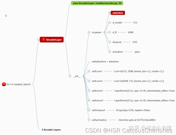
该图中展现的核心attention还没有展开;其他的,两个卷积,两个Norm,以及一个dropout,一个gelu函数,都列出来了。
class EncoderLayer(nn.Module):
    def __init__(self, attention, d_model, d_ff=None, dropout=0.1, activation="relu"):
        super(EncoderLayer, self).__init__()
        d_ff = d_ff or 4*d_model
        self.attention = attention
        self.conv1 = nn.Conv1d(in_channels=d_model, out_channels=d_ff, kernel_size=1)
        self.conv2 = nn.Conv1d(in_channels=d_ff, out_channels=d_model, kernel_size=1)
        self.norm1 = nn.LayerNorm(d_model)
        self.norm2 = nn.LayerNorm(d_model)
        self.dropout = nn.Dropout(dropout)
        self.activation = F.relu if activation == "relu" else F.gelu

    def forward(self, x, attn_mask=None):
        # x [B, L, D]
        # x = x + self.dropout(self.attention(
        #     x, x, x,
        #     attn_mask = attn_mask
        # ))
        new_x, attn = self.attention(
            x, x, x,
            attn_mask = attn_mask
        )
        x = x + self.dropout(new_x)

        y = x = self.norm1(x)
        y = self.dropout(self.activation(self.conv1(y.transpose(-1,1))))
        y = self.dropout(self.conv2(y).transpose(-1,1))

        return self.norm2(x+y), attn
Encoder类是将前面定义的Encoder层和Distilling操作组织起来,形成一个Encoder模块。其中distilling层总比EncoderLayer少一层,即最后一层EncoderLayer后不再做distilling操作。
class Encoder(nn.Module):
    def __init__(self, attn_layers, conv_layers=None, norm_layer=None):
        super(Encoder, self).__init__()
        self.attn_layers = nn.ModuleList(attn_layers)
        self.conv_layers = nn.ModuleList(conv_layers) if conv_layers is not None else None
        self.norm = norm_layer

    def forward(self, x, attn_mask=None):
        # x [B, L, D]
        attns = []
        if self.conv_layers is not None:
            for attn_layer, conv_layer in zip(self.attn_layers, self.conv_layers):
                x, attn = attn_layer(x, attn_mask=attn_mask)
                x = conv_layer(x)
                attns.append(attn)
            x, attn = self.attn_layers[-1](x, attn_mask=attn_mask)
            attns.append(attn)
        else:
            for attn_layer in self.attn_layers:
                x, attn = attn_layer(x, attn_mask=attn_mask)
                attns.append(attn)

        if self.norm is not None:
            x = self.norm(x)

        return x, attns
EncoderStack : 多个Encoder和蒸馏层的组合
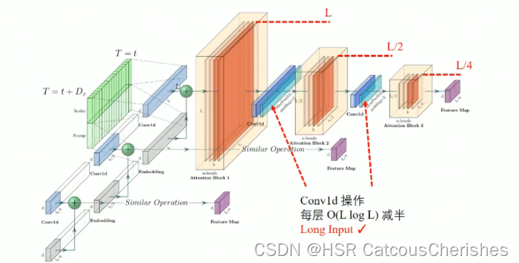
论文中有提到可以 采用多个replicas并行执行,不同replicas采用不同长度的embedding(L、L/2、L/4、…),embedding长度减半对应的attention层也减少一层,distilling层也会随之减少一层,最终得到的结果拼接起来作为输出(输出维度使对齐的)。
class EncoderStack(nn.Module):
    def __init__(self, encoders, inp_lens):
        super(EncoderStack, self).__init__()
        self.encoders = nn.ModuleList(encoders)
        self.inp_lens = inp_lens

    def forward(self, x, attn_mask=None):
        # x [B, L, D]
        x_stack = []; attns = []
        for i_len, encoder in zip(self.inp_lens, self.encoders):
            inp_len = x.shape[1]
            x_s, attn = encoder(x[:, -inp_len:, :])
            x_stack.append(x_s); attns.append(attn)
        x_stack = torch.cat(x_stack, -2)

        return x_stack, attns
到这里Encoder模块代码就差不多了,下一节继续Dencoder模块详情。
三. 总结
下一步是继续理解Decoder模块代码与整体model,并 构建自己的dataset去复现该LSTF问题在其他数据上的准确率,最好是可视化结果的对比。
毕设:提交初稿,根据老师意见,学弟正在修改。
Original: https://blog.csdn.net/weixin_44790306/article/details/124434860
Author: HSR CatcousCherishes
Title: CGAN—LSGAN的原理与实现与informer代码理解(1)
原创文章受到原创版权保护。转载请注明出处:https://www.johngo689.com/533022/
转载文章受原作者版权保护。转载请注明原作者出处!