语音识别初尝（DataWhale语音识别入门赛）

[天池ASR入门赛]语音识别初尝试

• 背景
  *
• ASR及语音相关的初认识
  –
  • 一些在我司常听到的关键词的介绍
    +
    *
    • 1）波形图
    • 2）采样点
    • 3）频谱图
  • 整体解决思路
  • 声学模型
  • 语言模型
  • 解码器
  • 端到端的方法
• 赛题及base-line的介绍
  *
• 赛题介绍
• 音频数据分析
  –
  • 声学特征介绍及提取
    +
  • 其他声学特征
  • MFCC特征抽取过程一个简介
  • MFCC抽取过程涉及到的内容
    *
    • 短时傅立叶变换
    • 梅尔谱
    • 关于py中MFCC的抽取使用
• 关于LSTM的baseline
  –
  • 简介
    +
  • 关于LSTM
  • 实现
• 改进模型方面的思路
  –
  • 过拟合与欠拟合
  • 拓展内容
    +
  • 语音识别的应用
  • 语音识别的开发工具
    *
    • 4.1 开源数据集
    • 4.2 开源语音识别项目

背景

这是第一次接触到语音识别的相关任务，本篇的笔记是对语音识别相应资料的个人直观理解，及datawhale的baseline解法的相关介绍
(豁免：真正主观的个人理解，可能涵盖错误)

[En]

(exemption: really subjective personal understanding, which may cover errors)

ASR及语音相关的初认识

一些在我司常听到的关键词的介绍

与文本不同，语音是看得见的，只有对应的音频，语音需要有一个“可见”的过程，所以有几种方式来表示音频文件如下：

[En]

Unlike text, speech can be seen, only the corresponding audio, there needs to be a “visible” process for speech, so there are several ways to represent audio files as follows:

1）波形图

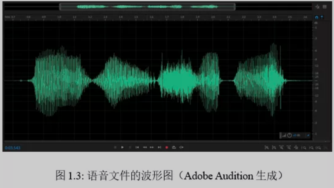
波形图：语音的保存形式可用波形图展现，可以看作是上下摆动的数字序列，每一秒的音频用16000个电压数值表示，采样率即为16kHz

; 2）采样点

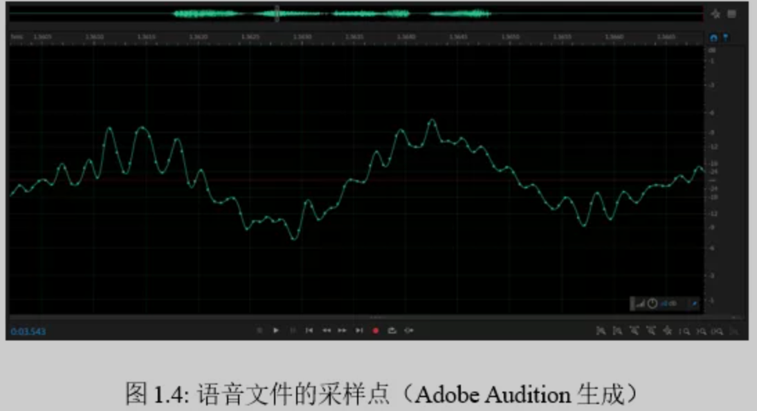
采样点：对波形图的放大，可以看到的更细的单位

3）频谱图

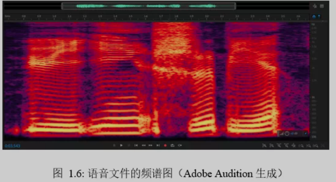
频谱图：可以变为 频谱图，颜色代表频带能量大小，语音的傅立叶变换是按帧进行，短的窗口有着高时域和低频域，长时窗口有低时域和高频域

基本单位
对于语音而言，基本单位是帧（对应文本的token），一帧即是一个向量，整条语音可以表示为以帧为单位的向量组。
帧是由ASR的前端声学特征提取模块产生，提取的技术设计”离散傅立叶变换”和”梅尔滤波器组”

; 整体解决思路

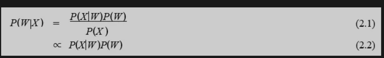
在我的理解认知中，对于ASR的解决方法可以分为两种，一种是声学模型加语言模型的组合，另外一种是端到端的解决方式。

第一种方式：
个人对路径的理解是，有一个音频，首先有一个声学模型，然后将对应的音频信号处理成对应的声学特征，然后使用语言模型从声学特征的结果中获得概率最高的输出串。

[En]

The personal understanding of the route is that there is an audio, first there is an acoustic model, and then the corresponding audio signal is processed into the corresponding acoustic feature, and then the language model is used to get the output string with the highest probability from the result of the acoustic feature.

在上图中， _X_代表的是声学特征向量， _W_代表输出的文本序列，在(2.1)中，P(X|W)代表的是声学模型，P(W)代表的是语言模型

第二种方式：
端到端的解决手段，个人印象中在吴恩达的课程里提到，ASR在CTC提出后有一个较大的提升。个人理解是在CTC之前，seq2seq的建模方式比较难处理输出序列远短于输入序列的情况，以及在不同帧出现的相同音素的输出

声学模型

常用的话，包括了HMM,GMM,DNN-HM的声学模型

语言模型

常用的语言模型这里包括了n-gram语言模型以及RNN的语言模型

解码器

最终目的是取得最大概率的字符输出，解码本质上是一个搜索问题，并可借助加权有限状态转换器（Weighted Finite State Transducer，WFST） 统一进行最优路径搜索.

端到端的方法

seq2seq+CTC 损失函数， RNN Transducer， Transforme，这里需要补充的话 应该要去看李宏毅2020年的人类语言处理的课程

赛题及base-line的介绍

比赛链接及介绍
（对榜首的99.95准确率表达amazing,怎么做到的…）

赛题介绍

介绍： 有20种不同食物的咀嚼声音，给出对应的音频，对声音的数据进行建模，判断是哪种食物的咀嚼声音

baseline思路：将对应的音频文件，使用librosa转化为梅尔谱作为输入的特征，用CNN对梅尔谱的特征进行建模分类预测。

较为重要的内容
1）关于librosa库
关于语音特征提取的库

[En]

A library about extracting speech features

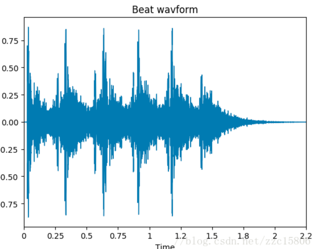
import librosa

y, sr = librosa.load('./beat.wav', sr=16000)

melspec = librosa.feature.melspectrogram(y, sr,
        n_fft=1024, hop_length=512, n_mels=128)

mfccs = librosa.feature.mfcc(y=y, sr=sr, n_mfcc=40)

import librosa.display
y, sr = librosa.load('./beat.wav', sr=None)
plt.figure()
librosa.display.waveplot(y, sr)
plt.title('Beat wavform')
plt.show()

相应的图片如下：

而基于base-line的实现中，就是将梅尔谱作为对应的cnn特征,

features = []
X, sample_rate = librosa.load(fn,res_type='kaiser_fast')
mels =np.mean(librosa.feature.melspectrogram(y=X,sr=sample_rate).T,axis=0)
feature.extend([mels])

推测这里的mean是做了一个正则化的操作

2）关于glob库
比较神奇的一个库，先前找文件夹下的文件可能会通过 os.path 结合是实现，通过该库是可以有一种比较优雅的方式获得文件夹中想要的文件

f = glob.iglob(r'../*.py')
for py in f:
    print py

而在其base-line中的显示使用

glob.glob(os.path.join(parent_dir, sub_dir, '.wav'))

3）关于tf.keras的建模方式
keras的建模方式还是比较便捷的
快速建模的核心的建模部分为通过Sequential，首先确定好输入的特征的维度，然后model.add()为模型添加上需要的模块（其实是比较好气说对于多输入特征的话这种方式work不work，要是有大佬看到的话，还是希望留言告知的）
通过model.compile模块将模型的结构固定，且在此时添加对应的损失函数及优化器等

model = Sequential()

input_dim = (16, 8, 1)

model.add(Conv2D(64, (3, 3), padding = "same", activation = "tanh", input_shape = input_dim))
model.add(MaxPool2D(pool_size=(2, 2)))
model.add(Conv2D(128, (3, 3), padding = "same", activation = "tanh"))
model.add(MaxPool2D(pool_size=(2, 2)))
model.add(Dropout(0.1))
model.add(Flatten())
model.add(Dense(1024, activation = "tanh"))
model.add(Dense(20, activation = "softmax"))

model.compile(optimizer = 'adam', loss = 'categorical_crossentropy', metrics = ['accuracy'])

对于训练和预测过程，则分别通过model.fit()和model.predict()完成

model.fit(X_train, Y_train, epochs = 20, batch_size = 15, validation_data = (X_test, Y_test))
predictions = model.predict(X_test.reshape(-1, 16, 8, 1))

音频数据分析

两个较为重要的库
对于音频文件，可用 librosa 和 PyAudio 进行一个语音特征的探索

在第一个库中，除了上面的波形，你还可以看到语音的另一个特征声图，它指的是声音随着时间的推移而产生的频谱的视觉表现(其实我仍然不太明白它的意思)。

[En]

In the first library, in addition to the above waveform, you can also see another feature of speech * sonogram * , which refers to a visual representation of the frequency spectrum of sound over time (in fact, I still don’t quite understand what it means).

频谱图的展示

plt.figure(figsize=(20, 10))
D = librosa.amplitude_to_db(np.abs(librosa.stft(data1)), ref=np.max)
plt.subplot(4, 2, 1)
librosa.display.specshow(D, y_axis='linear')
plt.colorbar(format='%+2.0f dB')
plt.title('Linear-frequency power spectrogram of aloe')

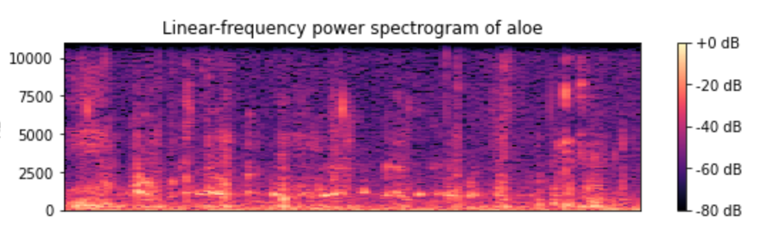
实际上，它代表了三维信息，水平轴代表时间，垂直轴代表频率，然后颜色深度代表声音的强度。

[En]

In fact, it represents the information of three dimensions, the horizontal axis represents time, the vertical axis represents frequency, and then the depth of color represents the intensity of sound.

而至于 PyAudio是为了让用户可以在交互的环境下，听对应的音频（但对于我这种.py用户来说 可能比较缺少实用性）

import IPython.display as ipd
ipd.Audio('./train_sample/aloe/24EJ22XBZ5.wav')

具有其他语音特征的名词简介：

[En]

Introduction to nouns with other phonetic features:

pitch: 称之为音调，以Hz为单位
基频： 称之为音高
能量：称之为音强

学习语音识别的一般过程如下：

[En]

The general process of learning about speech recognition:

1）静音切除，使用的手段包括了VAD
2) 声音分帧，通过滑动窗口实现，帧与帧之间会有交叉
3） 声学特征提取：通过线性预测倒谱系数（LPCC）和Mel 倒谱系数（MFCC），把每一帧的波形给转换为声学特征向量(类似于nlp中的embedding)?

4）声学模型：根据对应的声学特征，找到对应的音素信息
5）词典：由发音找到字词对应的token集合
6）语言模型：找到概率最大的输出字符序列
7）解码：过声学模型，字典，语言模型对提取特征后的音频数据进行文字输出。

声学特征介绍及提取

其他声学特征

过零率：是一个信号符号变化的比率，即语音信号由负变为正，由正变为负的次数，一般，过零率越高，频率越高

zero_crossings = librosa.zero_crossings(x[n0:n1], pad=False)

频谱质心： 用以描述音色属性，是频率成分的重心，是一定范围内通过能量加权平均的频率。

spectral_centroids = librosa.feature.spectral_centroid(x, sr=sr)[0]
print(spectral_centroids.shape)

frames = range(len(spectral_centroids))
t = librosa.frames_to_time(frames)

def normalize(x, axis=0):
    return sklearn.preprocessing.minmax_scale(x, axis=axis)

librosa.display.waveplot(x, sr=sr, alpha=0.4)

声谱衰减：是对声音信号形状（波形图）的一种衡量，表示低于总频谱能量的指定百分比的频率。

spectral_rolloff = librosa.feature.spectral_rolloff(x+0.01, sr=sr)[0]
librosa.display.waveplot(x, sr=sr, alpha=0.4)

MFCC特征抽取过程一个简介

MFCC: 是语音识别中常用的一种语音特征，提取的步骤如下

• 分帧
• 用周期图(periodogram) 法进行gong功率谱(power spercturm)的估计
• 对功率谱用Mel滤波器组进行滤波，计算每个滤波器里的能量
• 对每个滤波器的能量取log
• 进行离散余弦变换（DCT）变换
• 保留DCT的第2-13个系数，去掉其它
  前面两步是 短时傅立叶变换，后面几步主要涉及 *梅尔频谱

关于 短时傅立叶变换在干嘛：
首先涉及到 时域 与 频域 的概念，参照这里
时间域是时间和幅度的函数，而频域是频率和幅度的函数。(我认为这里的音乐例子更容易让人理解。)

[En]

Time domain is a function of time and amplitude, and frequency domain is a function of frequency and amplitude. (I think the examples of music here are easier for people to understand.)

个人的理解是，在单一的时间域中，我们缺少幅度(？)，仅仅看频域，我们失去了时间信息，所以我们需要一个工具来结合两者，然后在这里使用傅里叶变换。

[En]

Personal understanding is that in a single time domain, we lack amplitude (? ), just looking at the frequency domain, we lost the time information, so we need a tool to combine the two, and then the Fourier transform is used here.

这是DataWhale小姐姐的解释，所谓的短时傅里叶变换，即把一段长信号分帧、加窗，再对每一帧做快速傅里叶变换（FFT），最后把每一帧的结果沿另一个维度堆叠起来，得到类似于一幅图的二维信号形式。

MFCC抽取过程涉及到的内容

短时傅立叶变换

1）分帧：
将长语音切分为一个较为小的单位，个人认为是可以对接为nlp中的一个token，但为了连续性（？），不能帧跟帧之间完全的等分割裂，需要有一定的重合。我们通常以25ms为1帧，帧移为10ms，因此1秒的信号会有10帧。
2）对每帧信号做离散傅立叶变换（DFT）
这里…巴拉巴拉的放了一个公式… ，看不太懂到底干了啥… 累觉不爱（贴上一个 关于傅立叶变换的讲解，课后阅读）
可能是 将每一帧的信号 转换为 时域（？）
通过离散傅里叶变换得到声像图，其横坐标为帧下标，纵坐标为不同的频率或能量。图片中的颜色越暗(如红色)，相应频率的能量就越大。

[En]

The sonogram can be obtained from the discrete Fourier transform, its Abscissa is the frame subscript, and the ordinate is different frequency or energy. The darker the color in the picture (such as red), the greater the energy of the corresponding frequency.

在 librosa库，有对短时傅立叶变换的实现

y, sr = librosa.load('./train_sample/aloe/24EJ22XBZ5.wav')
S =librosa.stft(y, n_fft=2048, hop_length=None, win_length=None, window='hann', center=True, pad_mode='reflect')

S = np.abs(S)

梅尔谱

声谱图往往是很大的一张图，且依旧包含了大量无用的信息，所以我们需要通过梅尔标度滤波器组（mel-scale filter banks）将其变为梅尔频谱。
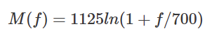
1） 梅尔尺度
更符合人类的听觉感知。从频率到MEL频率的转换公式如下：

[En]

Better match human auditory perception. The conversion formula from frequency to Mel frequency is as follows:

2）梅尔滤波器
为了模拟人耳对声音的感知，发明了梅尔滤波器组。一组大约20-40个(通常为26个)的三角形滤波器组，用于对上一步得到的周期图的功率谱估计进行滤波。间隔的频率越高，过滤器越宽(但如果将其变换为MEL比例，则宽度相同)。

[En]

In order to simulate the perception of sound by the human ear, the Mel filter bank was invented. A group of about 20-40 (usually 26) triangular filter banks that filter the power spectrum estimation of the periodic graph obtained in the previous step. And the higher the frequency of the interval, the wider the filter (but the same width if you transform it to the Mel scale).

（不知道这里的滤波器，其实是不是可以理解为类似于CNN的东西）

3）梅尔到谱
为了模拟人耳对声音的感知，发明了梅尔滤波器组。一组大约20-40个(通常为26个)的三角形滤波器组，用于对上一步得到的周期图的功率谱估计进行滤波。间隔的频率越高，过滤器越宽(但如果将其变换为MEL比例，则宽度相同)。

[En]

In order to simulate the perception of sound by the human ear, the Mel filter bank was invented. A group of about 20-40 (usually 26) triangular filter banks that filter the power spectrum estimation of the periodic graph obtained in the previous step. And the higher the frequency of the interval, the wider the filter (but the same width if you transform it to the Mel scale).

; 关于py中MFCC的抽取使用

在py中，可以通过librosa直接使用抽取MFCC的特征

mfccs = librosa.feature.mfcc(x, sr)
print (mfccs.shape)

librosa.display.specshow(mfccs, sr=sr, x_axis='time')

mfccs = sklearn.preprocessing.scale(mfccs, axis=1)

关于LSTM的baseline

简介

看到task4中其实是CNN中的模型base-line介绍，此时想看关于DataWhale的关于LSTM的代码介绍。对于ASR领域，应该是使用LSTM的情况会比较多一些？

关于LSTM

LSTM其实是RNN的一种变体，RNN的提出感觉整体上是为了解决时序问题数据的建模，即后续相对于RNN来讲，缓解了梯度爆炸和梯度消失的问题。
在给定的baseline中，是将音频文件中抽取队MFCC特征，继而将对应的特征，将每帧的MFCC特征传入到了LSTM中，由LSTM得到的hidden-state进入到两层的全连接层中。预测对应的标签概率。

实现

本文用的train_data.sample为例子

1）通过sox的指令可以将wav文件整理成16k的wav文件

sox file -b 16  -e signed-integer $new_dir"/"$file

2） 抽取MFCC特征的代码
由抽取出的MFCC的特征，存到文件中，后续写为json，由train.py的脚本读取进行训练。

def extract_mfcc(y, sr, size=1):
"""
    extract MFCC feature
    :param y: np.ndarray [shape=(n,)], real-valued the input signal (audio time series)
    :param sr: sample rate of 'y'
    :param size: the length (seconds) of random crop from original audio, default as 3 seconds
    :return: MFCC feature
"""

    y = y.astype(np.float32)
    normalization_factor = 1 / np.max(np.abs(y))
    y = y * normalization_factor

    melspectrogram = librosa.feature.melspectrogram(y=y, sr=sr, n_fft=2048, hop_length=1024)
    mfcc = librosa.feature.mfcc(S=librosa.power_to_db(melspectrogram), n_mfcc=20)
    mfcc_delta = librosa.feature.delta(mfcc)
    mfcc_delta_delta = librosa.feature.delta(mfcc_delta)
    mfcc_comb = np.concatenate([mfcc, mfcc_delta, mfcc_delta_delta], axis=0)

    return mfcc_comb

（在此将数据集的wav的文件及对应的特征写成json的写法感觉很值得借鉴）

4)关于训练的代码

核心的训练代码在此处

Solver/solver.py

看到train的代码是写在模型中的，逻辑上是造一个新的类，将数据，模型以及超参数，都作为类的一个属性，参与后续的训练代码的调用。

在它的类中，你可以找到一种方法来编写它，那就是，如果每一轮训练都很复杂，需要相应的返回，你可以在类中为每一轮编写一个方法，并重复调用。

[En]

In its class, you can find a way to write it, that is, if each training round is complicated and a corresponding return is needed, you can write a method in the class for each round and call it repeatedly.

for epoch in range(self.start_epoch, self.epochs):
    self.model.train()
    start = time.time()
    tr_avg_loss, _ = self._run_one_epoch(epoch)
    self.model.eval()
    val_loss, val_acc = self._run_one_epoch(epoch, cross_valid=True)

改进模型方面的思路

过拟合与欠拟合

粗糙定义：
过拟合：训练集上表现得好，测试集上表现的差
欠拟合：训练集和测试集都差
过拟合的应对思路：
1）加数据
也就是说，顾名思义，增加更多的数据，使模型不仅适应某种分布。

[En]

That is, as the name says, add more data to make the model not only adapt to a certain distribution.

2）砍模型
当模型很大，但数据规模很小时，我们需要从这个角度来考虑。

[En]

When the model is very large, but the data scale is small, we need to consider from this point of view.

3）正则化
这篇文章 是从损失函数的角度入手，例如我们拟合一条曲线时，如果各个次项的参数都学的比较好，完好的拟合了给定的曲线，会出现过拟合，此时我们希望说，低阶次项的影响小一些。所以损失函数会加上低阶的参数的值乘以一个较大的权重，这样loss-function在计算的时候，就会把对应的低阶项的参数值给减小。
当在神经网络中，我们不知道哪个参数需要乘以较大的权重，所以我们对所有参数的值采取范数，希望通过损失函数，模型会选择更重要的特征。

[En]

When in the neural network, we do not know which parameter needs to be multiplied by a larger weight, so we take the norm to the values of all parameters, hoping that through the loss function, the model will select the more important features.

这篇文章 讲了BN,LN之类的核心思想，大致的意思是，其实是做一个数据归一化的事情，既是为了尽量让中间的特征层呈现独立同分布的情况，BN为纵向的标准化，而LN为横向的标准化。
需要注意的是,就目前的实现来看，BN应该是可用在CNN类的网络，而LN适用在RNN类的网络
4）Dropout
NN的网络结构图中，某个计算节点，随机失活，减少输出层对某个节点的依赖
5) 集成模型
分为booosting和bagging，前者是基于分布和迭代。后者比较粗暴，基于多个分类器一起算，然后最后做投票，进行决策。
(深度学习的系统应该少用，玩游戏也可以。)

[En]

(it should be less used on the system with deep learning, and it is OK to play the game.)

(当时读书的时候，这两个人是不是不能做回归任务，只能做分类任务，我有点困惑。)

[En]

(when I was studying at that time, I was a little confused about whether these two could not do the regression task, but could only do the classification task.)

6) 损失函数加上floadding

loss = (loss - args.floadding_num).abs() + args.floadding_num

欠拟合的应对思路
缺乏拟合，一般来说，数据不够充分，网络设计不够好，或者现有功能不够，所以从以下三个角度进行改进

[En]

Lack of fitting, generally speaking, the data is not enough, the network design is not good enough, or the existing features are not enough, so it is improved from the following three angles

1）加特征：例如NLP加分词，加词性。
“在深度学习潮流中，有很多模型可以帮助完成特征工程，如因子分解机、梯度提升决策树、Deep-crossing等都可以成为丰富特征的方法”
2）扩大模型
3）考虑网络的设计是否合理

拓展内容

语音识别的应用

关键词检出（KWS，Keyword Spotting）， 唤醒词检测（Wake-up Word Detection，WUW）
声纹检测（VR，Voiceprint Recognition），说话人识别 （SR，Speaker Recognition）
语音识别（SR，Speech Recognition），语种识别（Spoken Language Recognition）

语音识别的开发工具

kaldi-asr/kaldi ： 支持的模型结构：GMM/CNN/LSTM/TDNN-HMM/LF-MMI/RNNLM
espnet Chainer/PyTorch：支持的模型结构：CTC/Attention/DNN-HMM/RNN-T

4.1 开源数据集

清华中文语音数据集THCHS-30
希尔贝壳中文普通话语音数据库AISHELL-2
中国明星声纹数据集 CN-Celeb2
kaldi中免费的数据集（中文跟英文）
Google发布的语音分离数据集
好未来开源近600小时中英文混合语音数据集
字节跳动发布全球最大钢琴MIDI数据集
中英文NLP数据集搜索库：CLUEDatasetSearch

4.2 开源语音识别项目

https://github.com/kaldi-asr/kaldi
https://github.com/SeanNaren/deepspeech.pytorch
https://github.com/srvk/eesen
https://github.com/Uberi/speech_recognition
https://github.com/xxbb1234021/speech_recognition

参考资料
李宏毅深度学习语音识别（2020最新版）
清语赋. 语音识别基本法
【概率图模型】 那些的你不知道的事
语音信号处理
传统语音识别（GMM+HMM）
GMM-HMM语音识别模型原理篇
马尔可夫链和隐马尔可夫模型
语音识别中的CTC算法的基本原理解释
Attention在语音识别中的应用
深度学习中的attention机制
语音交互评价指标
语音基础
语音识别的大致流程
DataWhale的github代码

Original: https://blog.csdn.net/weixin_41804613/article/details/115712889
Author: weixin_41804613
Title: 语音识别初尝（DataWhale语音识别入门赛）