

TensorFlow基本概念与常用函数
文章目录
- TensorFlow基本概念与常用函数
* - 一:张量
– - 二:常用函数
–
本人人工智能入门小白一枚,在网上学习人工智能实践-TensorFlow2.0(北大公开课)课程,将自己学习到的东西进行整理,为方便后面复习,如有错误,烦请指出!多谢!!
一:张量
(一):张量概念
TensorFlow 中的 Tensor 表示张量,即多维数组、多维列表,用阶表示张量的维数
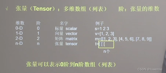

0 阶张量叫做标量,表示的是一个单独的数,如 123
1阶张量叫作向量,表示的是一个一维数组如[1,2,3]
2 阶张量叫作矩阵,表示的是一个二维数组,它可以有 i 行 j 列个元素,每个元素用它的行号和列号共同索引到,如在[[1,2,3],[4,5,6],[7,8,9]]中,2 的索引即为第 0 行第 1 列。
张量的阶数与方括号的数量相同,0 个方括号即为 0 阶张量,1 个方括号即为 1 阶张量。故张量可以表示 0阶到 n 阶的数组
; (二):TensorFlow中的数据类型
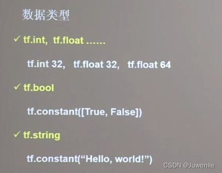
TensorFlow 中数据类型包括 32 位整型(tf.int32)、32 位浮点(tf.float32)、64 位浮点(tf.float64)、布尔型(tf.bool)、字符串型(tf.string)
(三):创建张量
1、利用tf.constant()
'''
创建张量
    tf.constant(张量内容,dtype=数据类型(可选))
'''
a = tf.constant([1,5],dtype=tf.int64)
print(a)
print(a.dtype)
print(a.shape)
利用 tf.constant(张量内容,dtype=数据类型(可选)),第一个参数表示张量内容,第二个参数表示张量的数据类型
输出结果:
<tf.Tensor([1,5], shape=(2 , ) , dtype=int64)>
<dtype: 'int64'>
(2,)
即会输出 张量内容、形状与数据类型,shape 中数字为 2,表示一维张量里有 2个元素。
注:去掉 dtype 项,不同电脑环境不同导致默认值不同,可能导致后续程序 bug
2、利用tf.convert_to_tensor()
很多时候数据是由 numpy 格式给出的,此时可以通过如下函数将 numpy 格式化为 Tensor 格式
'''
将numpy的数据类型转换成Tensor数据类型
    使用tf.convert_to_tensor(数据名,dtype=数据类型(可选))

'''
a = np.arange(0,5)
print(type(a))
b = tf.convert_to_tensor(a,dtype=tf.int64)
print(a)
print(b)

<class 'numpy.ndarray'>
[0 1 2 3 4]
tf.Tensor([0 1 2 3 4], shape=( 5 , ), dtype=int64)
可见,通过此函数将原本numpy格式的a数据转变成了Tensor的b数据
3、通过不同的函数来创建不同值的张量
用 tf. zeros(维度) 创建全为 0 的张量
用 tf.ones(维度) 创建全为 1 的张量
用 tf. fill(维度,指定值) 创建全为指定值的张量
注意:其中维度参数部分,如一维则直接写个数,二维用[行,列]表示,多维用[n,m,j…]
'''
创建张量
    创建全为0的张量
    tf.zeros(维度)

    创建全为1的张量
    tf.one(维度)

    创建指定值的张量
    tf.fill(维度,指定值)
'''
a = tf.zeros(4)
print(a)

b = tf.ones(2)
print(b)

c = tf.ones([2,3])
print(c)

d = tf.fill([2,3],4)
print(d)

tf.Tensor([0. 0. 0. 0.], shape=(4,), dtype=float32)

tf.Tensor([1. 1.], shape=(2,), dtype=float32)

tf.Tensor(
[[1. 1. 1.]
 [1. 1. 1.]], shape=(2, 3), dtype=float32)

tf.Tensor(
[[4 4 4]
 [4 4 4]], shape=(2, 3), dtype=int32)
注意:tf.zeros()、tf.ones()这两个函数产生的数据默认是浮点型,tf.fill()函数则会根据输入的数据来判断是什么类型
4、采用不同的函数创建符合不同分布的张量
- 生成 正态分布的随机数,默认均值为 0,标准差为 1
- tf. random.normal (维度,mean=均值,stddev=标准差)
- 生成 截断式正态分布的随机数
- tf. random.truncated_normal (维度,mean=均值,stddev=标准差)
- 生成 截断式正态分布的随机数,能使生成的这些随机数更集中一些,如果随机生成数据的取值在 (µ – 2 σ, u + 2 σ ) 之外则重新进行生成,保证了生成值在均值附近; µ:表示均值,σ:表示标准差
- 标准差的计算公式:
σ = ∑ i = 1 n ( x i − x ˉ ) 2 n \sigma = \sqrt{\frac{\sum_{i=1}^{n}{(x_i-\bar{x})}^2}{n}}σ=n ∑i =1 n (x i −x ˉ)2 - 生成 指定维度的均匀分布随机数
- tf. random. uniform(维度,minval=最小值,maxval=最大值)
- 生成指定维度的均匀分布随机数,用 minval 给定随机数的最小值,用 maxval 给定随机数的最大值,最小、最大值是 前闭后开区间
'''
创建随机张量
    生成正态分布的随机数。默认值为0,标准差为1
    tf.random.normal(维度,mean=均值,stddev =标准差)

    生成截断式正态分布的随机数
    tf.random.truncated_normal(维度,mean=均值,stddev=标准差)

    生成均匀分布的随机数
    tf.random.uniform(维度,minval=最小值,maxval=最大值)
'''
a = tf.random.normal([2,2],mean=0.5,stddev=1)
print(a)

b = tf.random.truncated_normal([2,2],mean=0.5,stddev=1)
print(b)

c = tf.random.uniform([2,2],minval=0,maxval=1)
print(c)

tf.Tensor(
[[1.0505471  0.45032525]
 [1.901815   0.4857818 ]], shape=(2, 2), dtype=float32)

tf.Tensor(
[[ 0.4339631  -0.23717612]
 [ 0.07864216  2.1449685 ]], shape=(2, 2), dtype=float32)

tf.Tensor(
[[0.6278517  0.34148467]
 [0.76214504 0.15577471]], shape=(2, 2), dtype=float32)
二:常用函数
(一):强制转换
利用 tf.cast (张量名,dtype=数据类型)强制将 Tensor 转换为该数据类型
'''
强制tensor转换成该数据类型
    tf.cast(张量名,dtype=数据类型)
'''
x1 = tf.constant([1.,2.,3.],dtype=tf.float64)
print(x1)
x2 = tf.cast(x1,tf.int64)
print(x2)

tf.Tensor([1. 2. 3.], shape=(3,), dtype=float64)
tf.Tensor([1 2 3], shape=(3,), dtype=int64)
(二):张量维度上的最值
'''
计算张量维中元素的最小值<details><summary>*<font color='gray'>[En]</font>*</summary>*<font color='gray'>Calculate the minimum value of an element in a tensor dimension</font>*</details>
    tf.reduce_min(张量名)

计算元素在张量维上的最大值<details><summary>*<font color='gray'>[En]</font>*</summary>*<font color='gray'>Calculate the maximum value of the element on the tensor dimension</font>*</details>
    tf.reduce_max(张量名)
'''
print(tf.reduce_min(x2),tf.reduce_max(x2))

tf.Tensor(1, shape=(), dtype=int64)   tf.Tensor(3, shape=(), dtype=int64)
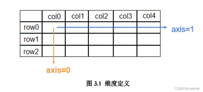
(三):理解axis
在一个二维张量或者数组中,可以通过调整axis等于0还是等于1来控制执行维度。
axis=0代表跨行(经度,down),而axis=1代表跨列(纬度,across)
如果不指定axis,则默认所有元素都参与计算
- 计算张量沿指定维度的平均值
[En]
calculate the average of the tensor along the specified dimension*
- tf.reduce_mean(张量名,axis=操作轴)
- 计算沿指定维度的张量和
[En]
calculate the sum of the tensor along the specified dimension*
- tf.reduce_sum(张量名,axis=操作轴)
x=tf.constant( [ [ 1, 2,3],[2, 2, 3] ] )print(x)print(tf.reduce_mean( x ))print(tf.reduce_sum( x, axis=1 ))tf.Tensor([[1 2 3] [2 2 3]], shape=(2, 3), dtype=int32)tf.Tensor(2, shape=(), dtype=int32) (对所有元素求均值)tf.Tensor([6 7], shape=(2,), dtype=int32) (横向求和,两行分别为 6 和 7)(四):标记变量为可训练
利用 tf.Variable(initial_value,trainable,validate_shape,name)函数可以将变量标记为”可训练”的,被它标记了的变量,会在反向传播中记录自己的梯度信息。
其中 initial_value 默认为 None,可以搭配 tensorflow 随机生成函数来初始化参数;
trainable 默认为 True,表示可以后期被算法优化的,如果不想该变量被优化,即改为 False;
validate_shape 默认为 True,形状不接受更改,如果需要更改,validate_shape=False;
name 默认为 None,给变量确定名称。
w = tf.Variable(tf.random.normal([2,2],mean=0,stddev=1))
print(w)

<tf.Variable 'Variable:0' shape=(2, 2) dtype=float32, numpy=
array([[ 1.3795949 ,  0.15414491],
       [-0.33091652, -0.03092775]], dtype=float32)>
我们训练一个网络,实际上是用数据来训练网络中的权值和阈值,以达到合适的状态并使误差最小化,所以在初始化权值后,我们必须将初始化后的随机权值标记为可训练的,以便在反向传播中通过梯度下降来更新权值。
[En]
We train a network, in fact, we use data to train the weights and thresholds in the network to achieve an appropriate state and minimize the error, so after we initialize the weights, we have to mark the initialized random weights as trainable, so that the weights can be updated by gradient descent in back propagation.
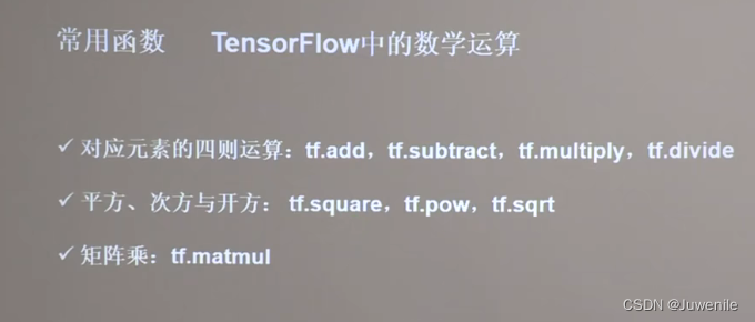
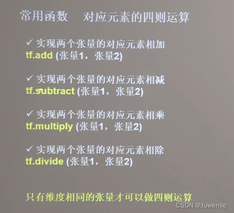
(五):常用的数学运算函数
; 1、四则运算
a = tf.ones([1,3])
b = tf.fill([1,3],3.)
print(a)
print(b)
print(tf.add(a,b))
print(tf.subtract(a,b))
print(tf.multiply(a,b))
print(tf.divide(a,b))

tf.Tensor([[1. 1. 1.]], shape=(1, 3), dtype=float32)
tf.Tensor([[3. 3. 3.]], shape=(1, 3), dtype=float32)
tf.Tensor([[4. 4. 4.]], shape=(1, 3), dtype=float32)
tf.Tensor([[-2. -2. -2.]], shape=(1, 3), dtype=float32)
tf.Tensor([[3. 3. 3.]], shape=(1, 3), dtype=float32)
tf.Tensor([[0.33333334 0.33333334 0.33333334]], shape=(1, 3), dtype=float32)
只有维度相同的张量才能够做四则运算
2、平方、次方与开方
- 计算某个张量的平方
- tf.square(张量名)
- 计算某个张量的n次方
- tf.pow(张量名,n次方数)
- 计算某个张量的开放
- tf.sqrt(张量名)
'''
平方、次方与开方
计算某个张量的平方
    tf.square(张量名)
计算某个张量的n次方
    tf.pow(张量名)
计算某个张量的开放
    tf.sqrt(张量名)
'''

c = tf.fill([1,2],3.)
print(c)
print(tf.square(c))
print(tf.pow(c,3))
print(tf.sqrt(c))

tf.Tensor([[3. 3.]], shape=(1, 2), dtype=float32)
tf.Tensor([[9. 9.]], shape=(1, 2), dtype=float32)
tf.Tensor([[27. 27.]], shape=(1, 2), dtype=float32)
tf.Tensor([[1.7320508 1.7320508]], shape=(1, 2), dtype=float32)
3、矩阵乘
- 实现两个矩阵的相乘
- tf.matmul(矩阵1,矩阵2)
'''
实现两个矩阵的相乘,矩阵乘法遵循3*2 x 2*3
    tf.matmul(矩阵1,矩阵2)
'''
a = tf.fill([2,3],3.)
b = tf.fill([3,2],2.)
print(a)
print(b)
print(tf.matmul(a,b))

tf.Tensor(
[[3. 3. 3.]
 [3. 3. 3.]], shape=(2, 3), dtype=float32)
tf.Tensor(
[[2. 2.]
 [2. 2.]
 [2. 2.]], shape=(3, 2), dtype=float32)
tf.Tensor(
[[18. 18.]
 [18. 18.]], shape=(2, 2), dtype=float32)
(六):特征与标签配对
可利用 tf.data.Dataset.from_tensor_slices((输入特征, 标签)) 切分传入张量的第一维度,生成 输入特征/标签对,构建数据集,此函数对Tensor 格式与 Numpy格式均适用,其切分的是第一维度,表征数据集中数据的数量,之后切分 batch等操作都以第一维为基础。
'''
神经网络在训练时,是把输入特征和标签配对后喂入网络的,所以tf给出了一种把特征和标签配对的函数
tf.data.Dataset.form_tensor_slices
Numpy和Tensor格式的数据都可以使用该条语句读入数据
'''
features = tf.constant([12,23,10,17])
labels = tf.constant([0,1,1,0])
dataset = tf.data.Dataset.from_tensor_slices((features,labels))
print(dataset)
for element in dataset:
    print(element)

<TensorSliceDataset element_spec=(TensorSpec(shape=(), dtype=tf.int32, name=None), TensorSpec(shape=(), dtype=tf.int32, name=None))>
(<tf.Tensor: shape=(), dtype=int32, numpy=12>, <tf.Tensor: shape=(), dtype=int32, numpy=0>)
(<tf.Tensor: shape=(), dtype=int32, numpy=23>, <tf.Tensor: shape=(), dtype=int32, numpy=1>)
(<tf.Tensor: shape=(), dtype=int32, numpy=10>, <tf.Tensor: shape=(), dtype=int32, numpy=1>)
(<tf.Tensor: shape=(), dtype=int32, numpy=17>, <tf.Tensor: shape=(), dtype=int32, numpy=0>)
'''
可见特征值 12 与标签0进行配对,特征值 23 与标签1进行配对,同理后面特征
'''
(七):计算损失函数在某一张量处的梯度
利用 tf.GradientTape( )函数搭配 with 结构计算损失函数在某一张量处的梯度
'''
gradient 求出张量的梯度
    gradient(函数,对谁求导)

'''
with tf.GradientTape() as tape:
    w = tf.Variable(tf.constant(3.0))
    loss = tf.pow(w,2)
grade = tape.gradient(loss,w)
print(grade)

tf.Tensor(6.0, shape=(), dtype=float32)
在上例中损失函数为:
l o s s = w 2 loss = w^{2}l oss =w 2
且当前w的取值是3,那么通过tape.gradient(loss,w)函数,将loss函数对w进行求导:即
∂ w 2 ∂ w = 2 w = 6 \frac{\partial w^2}{\partial w}=2w = 6 ∂w ∂w 2 =2 w =6
(八):枚举
enumerate是python的内建函数,它可以遍历每个元素(如:列表、元组或字符串)并在元素前配上对应的索引号,常在 for 循环中使用。
'''
枚举类型:
enumerate
'''
seq = ['one','two','three','four']
for i,element in enumerate(seq):
    print(i,element)

0 one
1 two
2 three
3 four
(九):独热码表示
什么是独热码:独热码
独热编码(one-hot encoding):在分类问题中,常用独热编码做标签,标签类别:1表示是,0表示非
用 tf.one_hot(待转换数据,depth=几分类) 函数实现用独热码表示标签,在分类问题中很常见,标记类别为为 1 和 0,其中 1 表示是,0 表示非。如在鸢尾花分类任务中,如果标签是 1,表示分类结果是 1 杂色鸢尾,其用把它用独热码表示就是 0,1,0,这样可以表示出每个分类的概率:也就是百分之 0 的可能是 0狗尾草鸢尾,百分百的可能是 1 杂色鸢尾,百分之 0 的可能是弗吉尼亚鸢尾。
'''
独热码
    tf.one_hot()函数将待转换数据转换为one-hot形式的数据输出
    tf.one_hot(待转换数据,depth=几分类)
'''
classes = 3
labels = tf.constant([1,0,2])
output = tf.one_hot(labels,depth=classes)
print(output)

tf.Tensor(
[[0. 1. 0.]
 [1. 0. 0.]
 [0. 0. 1.]], shape=(3, 3), dtype=float32)
为何会出现上述情况的结果呢?因为张量中数据的最小值是0,最大值是2,也就是说,值可能是1 PM/2 PM/3,0可以是100,0可以是10,1可以是0,2可以是0 01,所以结果如上所示。
[En]
Why is this the result of the above cases? Because the minimum of the data in the tensor is 0 and the maximum is 2, that is, the value may be 1pm / 2pm / 3. You can make 100 for 0, 0 10 for 1, and 0 01 for 2, so the result is shown above.
另外,索引是从0开始的,待转换数据中各元素值应小于 depth,若带转换元素值大于等于depth,则该元素输出编码为 [0, 0 … 0, 0]。即depth 确定列数,待转换元素的个数确定行数。
classes = 3
labels = tf.constant([1,4,2])
output = tf.one_hot(labels,depth=classes)
print(output)

tf.Tensor([[0. 1. 0.] [0. 0. 0.] [0. 0. 1.]], shape=(3, 3), dtype=float32)
(十):softmax()
利用 tf.nn.softmax( )函数使前向传播的输出值符合概率分布,进而与独热码形式的标签作比较
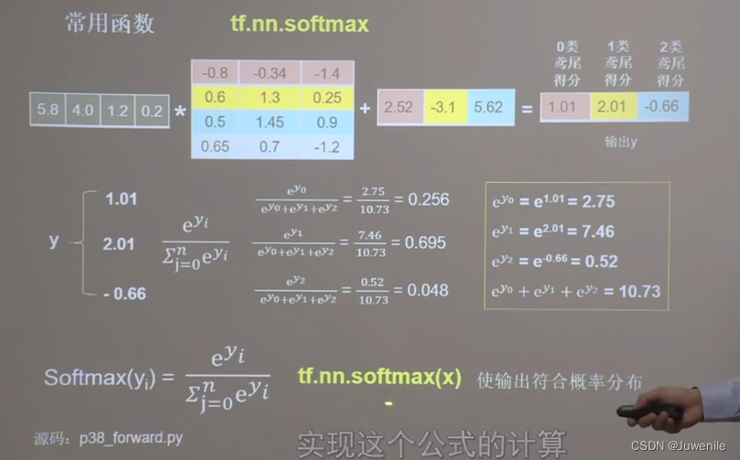
从上图可以看出,我们已经能够计算出预传播的输出值,分别为1.01、2.01和0.66。我们可以使用公式:
[En]
As can be seen from the figure above, we have been able to calculate the output values of pre-propagation, which are 1.01, 2.01, and 0.66, respectively. We can use the formula:
e y i ∑ j = 0 n e y i \frac{e^{y_i}}{\sum_{j=0}^{n}{e^{y_i}}}∑j =0 n e y i e y i
来计算出对应的概率值,其中yi就是前向传播的输出值。
'''
tf.nn.softmax()
该函数使输出数据符合概率分布。<details><summary>*<font color='gray'>[En]</font>*</summary>*<font color='gray'>This function makes the output data conform to the probability distribution.</font>*</details>
'''
y = tf.constant([1.01,2.01,-0.66])
y_pro = tf.nn.softmax(y)
print(y_pro)

tf.Tensor([0.25598174 0.69583046 0.04818781], shape=(3,), dtype=float32)
结果的概率值相加为1
(十一):实现自更新
利用 assign_sub()函数 对参数实现自更新,更新参数的值并返回,在使用此函数前需利用 tf.Variable定义变量 _w_为可训练(可自更新)
'''
自减操作
在使用assign_sub函数前,先用tf.Variable定义变量为可训练的
w.assign_sub(要自减的内容)
'''
w = tf.Variable(4)
w.assign_sub(1)
print(w)

<tf.Variable 'Variable:0' shape=() dtype=int32, numpy=3>
注:直接调用 tf.assign_sub 会报错,要用 w.assign_sub。
(十二):tf.argmax()函数
利用 tf.argmax (张量名,axis=操作轴) 返回张量沿指定维度最大值的索引
'''
返回沿指定维度的最大张量的索引<details><summary>*<font color='gray'>[En]</font>*</summary>*<font color='gray'>Returns the index of the maximum tensor along the specified dimension</font>*</details>
tf.argmax(张量名,axis=操作轴)
'''
test = np.array([[1,2,3],[2,3,4],[5,4,3],[8,7,2]])
print(test)
print(tf.argmax(test,axis=0))
print(tf.argmax(test,axis=1))

[[1 2 3]
 [2 3 4]
 [5 4 3]
 [8 7 2]]
tf.Tensor([3 3 1], shape=(3,), dtype=int64)
tf.Tensor([2 2 0 0], shape=(4,), dtype=int64)
Original: https://blog.csdn.net/weixin_43288447/article/details/126274568
Author: Juwenile
Title: TensorFlow基本概念与常用函数
原创文章受到原创版权保护。转载请注明出处:https://www.johngo689.com/513916/
转载文章受原作者版权保护。转载请注明原作者出处!