

mask r-cnn 代码解读(一)
文章目录
- 1 代码架构
- 2 model.py 的结构
- 3 train过程代码解析
* - 3.1 Resnet Graph
- 3.2 Region Proposal Network (RPN)
- 3.3 Proposal Layer
本系列将对 mask r-cnn 的代码做非常详细的讲解。
默认教程使用者已经对mask r-cnn的结构基本了解,因此不对原论文做解析
、最好是读者手头有完整的mrcnn代码(没有也没事,会贴),对照着代码和博客来理解。
本文将通过对代码的解析,重新梳理网络结构中的歧义。
[En]
This article will sort out the ambiguities in the network structure again by parsing the code.
1 代码架构
如下图所示,mrcnn 中包含四个主要的python文件:
config,py:代码中涉及的超参数放在此文件中model.py:深度网络的build代码utils.py:涉及一些工具方法visualize.py:预测(detect)得到结果后,将预测的Bbox和mask结合原图重新绘制
另外还有parallel_model.py,是为了方便模型在多GPU上训练。


本文将主要根据model.py的内容进行,此过程中调用了别的代码时,也会对被调用的解析。
; 2 model.py 的结构
model.py 特别长,可根据内容划分成如下块:
块作用Utility Functions对日志记录等做一些规定Resnet Graph基础网络,提取特征(feature)Region Proposal Network (RPN)在feature上生成anchors,并给出粗略的前景/背景判断结果、粗略的Bbox坐标Proposal Layer输入rpn网络得到的Bbox,过滤背景得到proposalsROIAlign Layer输入基础网络提取到的特征和 rois 的坐标,剪裁得到特征上坐标对应的部分。并reshape到相同大小Detection Target Layertrain过程中,根据ground truth 和 proposal得到 rois(region of interest)Detection Layerinference过程中,根据proposals和Bbox deltas得到最后的Bbox结果Feature Pyramid Network Heads输入pool后的特征,预测物体class和maskMaskRCNN Class将上述结构串起来,最后返回一个model对象Loss Functions损失函数相关Data Generator管理训练数据等Data Formatting对输入图片的一些处理Miscellenous Graph Functions其他一些函数
接下来将按照 Resnet Graph → RPN → Proposal Layer → ROIAlign Layer → Detection Target Layer → Feature Pyramid Network Heads → MaskRCNN Class 的顺序讲解 train 部分的代码。
然后是 inference 中不同的代码部分。
然后是丢失功能和数据优先操作。
[En]
Then there is the loss function and data first off operation.
整个解析中,会:
- 贴上增加注释的代码
- 将代码转换为易于理解的流程图
[En]
convert the code into an easy-to-understand flowchart*
- 对代码中不易理解/别扭(个人认为)的地方额外解释
3 train过程代码解析
3.1 Resnet Graph
这部分代码比较简单,网络结构也很清晰。有三种方法:
[En]
This part of the code is relatively simple, and the network structure is very clear. There are three methods:
- def identity_block
- def conv_block
- def resnet_graph
其中 identity_block 和 conv_block 是定义的两个卷积块,也就是两种不同的卷积方式:


具体的代码也贴在下方:
def identity_block(input_tensor, kernel_size, filters, stage, block,
                   use_bias=True, train_bn=True):
    """The identity_block is the block that has no conv layer at shortcut
    # Arguments
        input_tensor: input tensor
        kernel_size: default 3, the kernel size of middle conv layer at main path
        filters: list of integers, the nb_filters of 3 conv layer at main path
        stage: integer, current stage label, used for generating layer names
        block: 'a','b'..., current block label, used for generating layer names
        use_bias: Boolean. To use or not use a bias in conv layers.

        train_bn: Boolean. Train or freeze Batch Norm layers
"""
    '''
    一个1x1卷积 → 一个kxk卷积(kernel size) → 一个1x1卷积 → 卷积结果和input加起来(像素相加)
    '''
    nb_filter1, nb_filter2, nb_filter3 = filters
    conv_name_base = 'res' + str(stage) + block + '_branch'
    bn_name_base = 'bn' + str(stage) + block + '_branch'

    x = KL.Conv2D(nb_filter1, (1, 1), name=conv_name_base + '2a',
                  use_bias=use_bias)(input_tensor)
    x = BatchNorm(name=bn_name_base + '2a')(x, training=train_bn)
    x = KL.Activation('relu')(x)

    x = KL.Conv2D(nb_filter2, (kernel_size, kernel_size), padding='same',
                  name=conv_name_base + '2b', use_bias=use_bias)(x)
    x = BatchNorm(name=bn_name_base + '2b')(x, training=train_bn)
    x = KL.Activation('relu')(x)

    x = KL.Conv2D(nb_filter3, (1, 1), name=conv_name_base + '2c',
                  use_bias=use_bias)(x)
    x = BatchNorm(name=bn_name_base + '2c')(x, training=train_bn)

    x = KL.Add()([x, input_tensor])
    x = KL.Activation('relu', name='res' + str(stage) + block + '_out')(x)
    return x

def conv_block(input_tensor, kernel_size, filters, stage, block,
               strides=(2, 2), use_bias=True, train_bn=True):
    """conv_block is the block that has a conv layer at shortcut
    # Arguments
        input_tensor: input tensor
        kernel_size: default 3, the kernel size of middle conv layer at main path
        filters: list of integers, the nb_filters of 3 conv layer at main path
        stage: integer, current stage label, used for generating layer names
        block: 'a','b'..., current block label, used for generating layer names
        use_bias: Boolean. To use or not use a bias in conv layers.

        train_bn: Boolean. Train or freeze Batch Norm layers
    Note that from stage 3, the first conv layer at main path is with subsample=(2,2)
    And the shortcut should have subsample=(2,2) as well
"""
    '''
    一个1x1卷积 → 一个kxk卷积(kernel size) → 一个1x1卷积 → 卷积结果和input 1x1卷积后 加起来(像素相加)
    '''
    nb_filter1, nb_filter2, nb_filter3 = filters
    conv_name_base = 'res' + str(stage) + block + '_branch'
    bn_name_base = 'bn' + str(stage) + block + '_branch'

    x = KL.Conv2D(nb_filter1, (1, 1), strides=strides,
                  name=conv_name_base + '2a', use_bias=use_bias)(input_tensor)
    x = BatchNorm(name=bn_name_base + '2a')(x, training=train_bn)
    x = KL.Activation('relu')(x)

    x = KL.Conv2D(nb_filter2, (kernel_size, kernel_size), padding='same',
                  name=conv_name_base + '2b', use_bias=use_bias)(x)
    x = BatchNorm(name=bn_name_base + '2b')(x, training=train_bn)
    x = KL.Activation('relu')(x)

    x = KL.Conv2D(nb_filter3, (1, 1), name=conv_name_base +
                  '2c', use_bias=use_bias)(x)
    x = BatchNorm(name=bn_name_base + '2c')(x, training=train_bn)

    shortcut = KL.Conv2D(nb_filter3, (1, 1), strides=strides,
                         name=conv_name_base + '1', use_bias=use_bias)(input_tensor)
    shortcut = BatchNorm(name=bn_name_base + '1')(shortcut, training=train_bn)

    x = KL.Add()([x, shortcut])
    x = KL.Activation('relu', name='res' + str(stage) + block + '_out')(x)
    return x
在 resnet_graph 中,调用这两种卷积块,得到特征图。
首先:
def resnet_graph(input_image, architecture, stage5=False, train_bn=True):
    """Build a ResNet graph.

        architecture: Can be resnet50 or resnet101
        stage5: Boolean. If False, stage5 of the network is not created
        train_bn: Boolean. Train or freeze Batch Norm layers
"""
    assert architecture in ["resnet50", "resnet101"]
assert 是断言,如果输入的architecture不是resnet50或者resnet101中某一个的话,将报错。
然后调用上述两个卷积块进行特征提取。
[En]
Then the above two convolution blocks are called for feature extraction.
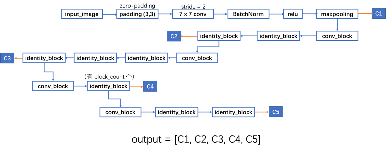
def resnet_graph(input_image, architecture, stage5=False, train_bn=True):
    ...

    x = KL.ZeroPadding2D((3, 3))(input_image)
    x = KL.Conv2D(64, (7, 7), strides=(2, 2), name='conv1', use_bias=True)(x)
    x = BatchNorm(name='bn_conv1')(x, training=train_bn)
    x = KL.Activation('relu')(x)
    C1 = x = KL.MaxPooling2D((3, 3), strides=(2, 2), padding="same")(x)

    x = conv_block(x, 3, [64, 64, 256], stage=2, block='a', strides=(1, 1), train_bn=train_bn)
    x = identity_block(x, 3, [64, 64, 256], stage=2, block='b', train_bn=train_bn)
    C2 = x = identity_block(x, 3, [64, 64, 256], stage=2, block='c', train_bn=train_bn)

    x = conv_block(x, 3, [128, 128, 512], stage=3, block='a', train_bn=train_bn)
    x = identity_block(x, 3, [128, 128, 512], stage=3, block='b', train_bn=train_bn)
    x = identity_block(x, 3, [128, 128, 512], stage=3, block='c', train_bn=train_bn)
    C3 = x = identity_block(x, 3, [128, 128, 512], stage=3, block='d', train_bn=train_bn)

    x = conv_block(x, 3, [256, 256, 1024], stage=4, block='a', train_bn=train_bn)
    block_count = {"resnet50": 5, "resnet101": 22}[architecture]
    for i in range(block_count):
        x = identity_block(x, 3, [256, 256, 1024], stage=4, block=chr(98 + i), train_bn=train_bn)
    C4 = x

    if stage5:
        x = conv_block(x, 3, [512, 512, 2048], stage=5, block='a', train_bn=train_bn)
        x = identity_block(x, 3, [512, 512, 2048], stage=5, block='b', train_bn=train_bn)
        C5 = x = identity_block(x, 3, [512, 512, 2048], stage=5, block='c', train_bn=train_bn)
    else:
        C5 = None
    return [C1, C2, C3, C4, C5]
这部分代码也很简单,基本上是直截了当的,整理出这部分的网络结构如下:
[En]
This part of the code is also very simple, basically straightforward, sort out this part of the network structure is as follows:
3.2 Region Proposal Network (RPN)
这部分包括两个方法:
- def rpn_graph(feature_map, anchors_per_location, anchor_stride)
- def build_rpn_model(anchor_stride, anchors_per_location, depth)
在 build_rpn_graph 中调用 rpn_graph ,得到output然后返回一个model对象。(先在 **_graph 方法中写好网络结构,然后在 build_** 方法中调用它,返回一个model对象。这种写代码思路是CNN中常见的写法。后文不再提及。 )
其中输入参数说明如下:
feature_map,shape = [batch, height, width, depth],是上文 resnet 输出的结果。anchors_per_location:feature 中每个 pixel 产生的 anchors 的数量anchor_stride:产生anchors的间隔,一般是1(也就是每个pixel都产生anchors),或者2(间隔一个)
需要说明的是,之前 resnet 产生了五个不同尺寸的 feature ,而 RPN 的输入中没有体现这一点。
这是因为:在后期 Mask RCNN 调用这两个 layer 的时候,将 resnet 生成的 feature 放入 list 中,然后循环 list ,对每一层的 feature 单独输入 RPN。
返回:
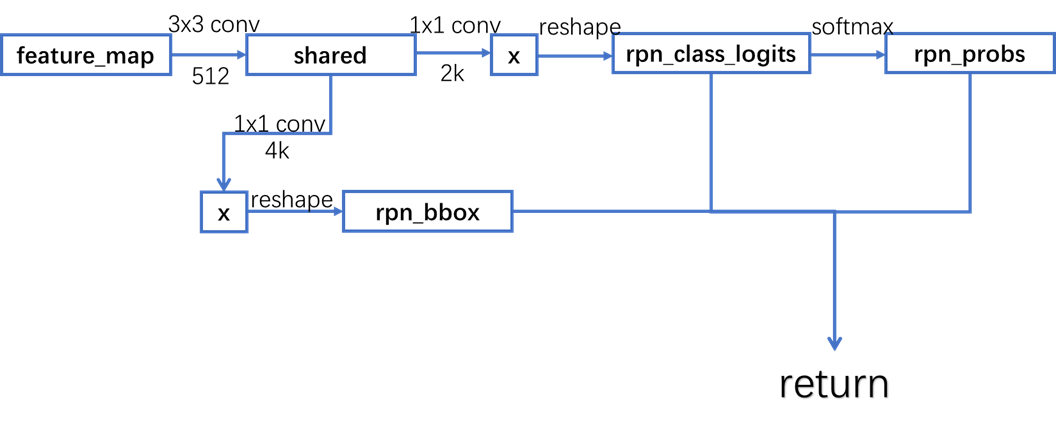
rpn_class_logits,shape = [batch, H * W * anchors_per_location, 2] 这个是anchors 分类结果激活前的张量。rpn_probs,shape = [batch, H * W * anchors_per_location, 2] 这是上面logits激活(softmax)之后的结果,表示 anchor 分类结果的得分。(或者说可能性,probs就是probabilities)shape中最后一维是”2″,代表 前景(有对象)/背景 的初步判断结果。rpn_bbox,shape = [batch, H * W * anchors_per_location, 4],最后一维的4具体是 (dy, dx, log(dh), log(dw))。这是anchors回归的delta。
具体代码如下:
def rpn_graph(feature_map, anchors_per_location, anchor_stride):
    """Builds the computation graph of Region Proposal Network.

    feature_map: backbone features [batch, height, width, depth]
    anchors_per_location: number of anchors per pixel in the feature map
    anchor_stride: Controls the density of anchors. Typically 1 (anchors for
                   every pixel in the feature map), or 2 (every other pixel).

    Returns:
        rpn_class_logits: [batch, H * W * anchors_per_location, 2] Anchor classifier logits (before softmax)
        rpn_probs: [batch, H * W * anchors_per_location, 2] Anchor classifier probabilities.

        rpn_bbox: [batch, H * W * anchors_per_location, (dy, dx, log(dh), log(dw))] Deltas to be
                  applied to anchors.

"""

    shared = KL.Conv2D(512, (3, 3), padding='same', activation='relu',
                       strides=anchor_stride,
                       name='rpn_conv_shared')(feature_map)

    x = KL.Conv2D(2 * anchors_per_location, (1, 1), padding='valid',
                  activation='linear', name='rpn_class_raw')(shared)

    rpn_class_logits = KL.Lambda(
        lambda t: tf.reshape(t, [tf.shape(t)[0], -1, 2]))(x)

    rpn_probs = KL.Activation(
        "softmax", name="rpn_class_xxx")(rpn_class_logits)

    x = KL.Conv2D(anchors_per_location * 4, (1, 1), padding="valid",
                  activation='linear', name='rpn_bbox_pred')(shared)

    rpn_bbox = KL.Lambda(lambda t: tf.reshape(t, [tf.shape(t)[0], -1, 4]))(x)

    return [rpn_class_logits, rpn_probs, rpn_bbox]
选其中稍微别扭的解释:
rpn_class_logits = KL.Lambda(
        lambda t: tf.reshape(t, [tf.shape(t)[0], -1, 2]))(x)
其中 x 是 feature_map 经过一个 3×3 卷积(padding)之后得到 share、再经过 1×1 卷积的结果,feature_map 的 shape=[batch, w, h, channel],share 的 shape=[batch, w, h, channel=512]。
所以 x.shape = [batch, w, h, 2k](k指每个pixel产生几个anchor,系数2是因为要划分前景和背景)。
x 是 rpn_class_logits 的前身,shape 需要变成 [batch, hwk, 2],这个好理解。
这句话的含义就等价于:
def function(x):
    batch = x.shape[0]
    result = tf.reshape(x, [batch, -1, 2])

    return result

rpn_class_logits = function(x)
那么又有一个新问题:为什么不按照我这个写法,而是用 KL.Lambda 呢?
(这并不是因为它太简洁了。你好)
[En]
(it’s not because it’s so concise. Hello)
因为 keras 的数据流可以被 tensorflow 直接处理,但是 tensorflow 出来的东西,keras 就不认了……在这个例子中, tf.reshape(x, [batch, -1, 2]) 就是从 tensorflow 出来的数据流,没办法被 keras 直接处理。
一种简单的解决方案是: 引入Keras的Lamda函数将TensorFlow的操作转化为Keras的数据流。这样就可以将TensorFlow写好的函数输出直接转换为Keras的Module可以接收的类型。
(下文还会提到另一种解决方案:继承Layer,重写一个类)
结构图可以从代码中获得,如下所示:
[En]
The structure diagram can be obtained from the code as follows:
3.3 Proposal Layer
本节定义了两个函数和一个类:
[En]
This section defines two functions and a class:
- def apply_box_deltas_graph(boxes, deltas)
- def clip_boxes_graph(boxes, window)
- class ProposalLayer(KE.Layer)
前两个方法是工具方法, apply_box_deltas_graph 输入 Bbox 坐标和 delta ,输出根据delta 精调后的 Bbox。 clip_boxes_graph 输入 bbox 和 window ,输出这两个区域的重合部分的坐标。
诶……那么这个 window 是什么呢?
在 Data Formatting 的部分中,有两个函数:
- def compose_image_meta:对原始图像信息打包
- def parse_image_meta(meta):对原始图像信息解包
这两个代码非常容易理解,并直接发布在下面:
[En]
These two codes are very easy to understand and are posted directly below:
def compose_image_meta(image_id, original_image_shape, image_shape,
                       window, scale, active_class_ids):
    """Takes attributes of an image and puts them in one 1D array.

    image_id: An int ID of the image. Useful for debugging.

    original_image_shape: [H, W, C] before resizing or padding.

    image_shape: [H, W, C] after resizing and padding
    window: (y1, x1, y2, x2) in pixels. The area of the image where the real
            image is (excluding the padding)
    scale: The scaling factor applied to the original image (float32)
    active_class_ids: List of class_ids available in the dataset from which
        the image came. Useful if training on images from multiple datasets
        where not all classes are present in all datasets.

"""
    meta = np.array(
        [image_id] +
        list(original_image_shape) +
        list(image_shape) +
        list(window) +
        [scale] +
        list(active_class_ids)
    )
    return meta

def parse_image_meta(meta):
    """Parses an array that contains image attributes to its components.

    See compose_image_meta() for more details.

    meta: [batch, meta length] where meta length depends on NUM_CLASSES

    Returns a dict of the parsed values.

"""
    image_id = meta[:, 0]
    original_image_shape = meta[:, 1:4]
    image_shape = meta[:, 4:7]
    window = meta[:, 7:11]
    scale = meta[:, 11]
    active_class_ids = meta[:, 12:]
    return {
        "image_id": image_id.astype(np.int32),
        "original_image_shape": original_image_shape.astype(np.int32),
        "image_shape": image_shape.astype(np.int32),
        "window": window.astype(np.int32),
        "scale": scale.astype(np.float32),
        "active_class_ids": active_class_ids.astype(np.int32),
    }
从这里就可以知道, window 是 原始图片 resize + padding 后,处理后的新图像中具有原始图像的部分。
但!是!在 ProposalLayer 的 call 方法调用这个函数的时候,是在归一化的坐标系里, 并没有从image_meta中读数据,而是:
window = np.array([0, 0, 1, 1], dtype=np.float32)
具体的 apply_box_deltas_graph 和 clip_boxes_graph 代码也贴在下面。(虽然跳过这个不会对理解mask rcnn造成影响)
def apply_box_deltas_graph(boxes, deltas):
    """Applies the given deltas to the given boxes.

    boxes: [N, (y1, x1, y2, x2)] boxes to update
    deltas: [N, (dy, dx, log(dh), log(dw))] refinements to apply
"""

    height = boxes[:, 2] - boxes[:, 0]
    width = boxes[:, 3] - boxes[:, 1]
    center_y = boxes[:, 0] + 0.5 * height
    center_x = boxes[:, 1] + 0.5 * width

    center_y += deltas[:, 0] * height
    center_x += deltas[:, 1] * width
    height *= tf.exp(deltas[:, 2])
    width *= tf.exp(deltas[:, 3])

    y1 = center_y - 0.5 * height
    x1 = center_x - 0.5 * width
    y2 = y1 + height
    x2 = x1 + width
    result = tf.stack([y1, x1, y2, x2], axis=1, name="apply_box_deltas_out")
    return result

def clip_boxes_graph(boxes, window):
"""
    保留交集的函数
    boxes: [N, (y1, x1, y2, x2)]
    window: [4] in the form y1, x1, y2, x2
"""

    wy1, wx1, wy2, wx2 = tf.split(window, 4)
    y1, x1, y2, x2 = tf.split(boxes, 4, axis=1)

    y1 = tf.maximum(tf.minimum(y1, wy2), wy1)
    x1 = tf.maximum(tf.minimum(x1, wx2), wx1)
    y2 = tf.maximum(tf.minimum(y2, wy2), wy1)
    x2 = tf.maximum(tf.minimum(x2, wx2), wx1)
    clipped = tf.concat([y1, x1, y2, x2], axis=1, name="clipped_boxes")
    clipped.set_shape((clipped.shape[0], 4))
    return clipped
然后是 Proposal Layer 的重点: ProposalLayer 类,它继承 keras.engine.Layer ,包括三个方法:
- def init
- def call
- def compute_output_shape
为什么要写一个类继承Layer,而不是直接 def 一个方法解决呢?跟上文提到使用 KL.Lambda 类似,TensorFlow的函数可以操作Keras的Tensor,但是它返回的TensorFlow的Tensor不能被Keras继续处理,因此我们需要:
建立新的Keras层进行转换,将TensorFlow的Tensor作为Keras层的__init__函数进行构建层,然后在__call__方法中使用TensorFlow的函数进行细粒度的数据处理,最后返回Keras层对象。
然后根据 Keras 的 API 文档,实现自己的类需要重写:
build(input_shape):这是定义权重的方法,可训练的权应该在这里被加入列表call(x):这是定义层功能的方法,除非你希望你写的层支持masking,否则你只需要关心call的第一个参数:输入张量compute_output_shape(input_shape):如果你的层修改了输入数据的shape,你应该在这里指定shape变化的方法,这个函数使得Keras可以做自动shape推断
诶那为什么只实现了 call 和 compute_output_shape(input_shape),而不见 build 的踪影呢?
我们点进keras的源代码:
    def build(self, input_shape):
        """Creates the layer weights.

        Must be implemented on all layers that have weights.

        # Arguments
            input_shape: Keras tensor (future input to layer)
                or list/tuple of Keras tensors to reference
                for weight shape computations.

"""
        self.built = True
注意,是所有有权重的层才要重写这个方法。那咱们 ProposalLayer 有权重吗?
没有!
所以不需要重写。
先看 __init__ 方法:
def __init__(self, proposal_count, nms_threshold, config=None, **kwargs):
        super(ProposalLayer, self).__init__(**kwargs)
        self.config = config
        self.proposal_count = proposal_count
        self.nms_threshold = nms_threshold
其中, proposal_count 是一个整数,用于指定生成proposal数目,不足时会生成坐标为[0,0,0,0]的空值进行补全。这个数由config文件中 POST_NMS_ROIS_TRAINING 或者 POST_NMS_ROIS_INFERENCE 决定。
nms_threshold 是非极大值抑制的阈值,由 config.RPN_NMS_THRESHOLD 决定,如果调大这个参数,会产生更多的proposals。
接下来重点看 call 方法的实现。其中输入参数是:
rpn_probs:[batch, num_anchors, 2],2具体是(bg prob, fg prob)。其中bg指 background,fg指 foregroundrpn_bbox:[batch, num_anchors, 4], 4具体是(dy, dx, log(dh), log(dw))anchors:[batch, num_anchors, 4], 4具体是(y1, x1, y2, x2)。坐标是在 normalized 的坐标系中的值。
返回:
- 在 normalized 的坐标系中的
proposals,shape=[batch, rois, 4],4具体是(y1, x1, y2, x2)
然后发布带注释的源代码:
[En]
Then post the annotated source code:
    def call(self, inputs):

        scores = inputs[0][:, :, 1]

        deltas = inputs[1]
        deltas = deltas * np.reshape(self.config.RPN_BBOX_STD_DEV, [1, 1, 4])

        anchors = inputs[2]

        pre_nms_limit = tf.minimum(self.config.PRE_NMS_LIMIT, tf.shape(anchors)[1])

        ix = tf.nn.top_k(scores, pre_nms_limit, sorted=True,
                         name="top_anchors").indices

        scores = utils.batch_slice([scores, ix], lambda x, y: tf.gather(x, y),
                                   self.config.IMAGES_PER_GPU)
        deltas = utils.batch_slice([deltas, ix], lambda x, y: tf.gather(x, y),
                                   self.config.IMAGES_PER_GPU)
        pre_nms_anchors = utils.batch_slice([anchors, ix], lambda a, x: tf.gather(a, x),
                                    self.config.IMAGES_PER_GPU,
                                    names=["pre_nms_anchors"])
        '''
        关于batch_slice: 这个函数将只支持batch为1的函数进行了扩展(实际就是不能有batch维度的函数),
        tf.gather函数只能进行一维数组的切片,而scares为2维[batch, num_rois],
        相对的ix也是二维[batch, top_k],所以我们需要将两者切片应用函数后将结果拼接。
        '''

        boxes = utils.batch_slice([pre_nms_anchors, deltas],
                                  lambda x, y: apply_box_deltas_graph(x, y),
                                  self.config.IMAGES_PER_GPU,
                                  names=["refined_anchors"])

        '''
        我们的锚框坐标实际上是位于一个归一化了的图上, 上一步的修正进行之后不再能够保证这一点,
        所以我们需要切除锚框越界的的部分(即只保留锚框和[0,0,1,1]画布的交集),通过调用clip_boxes_graph
        '''
        window = np.array([0, 0, 1, 1], dtype=np.float32)
        boxes = utils.batch_slice(boxes,
                                  lambda x: clip_boxes_graph(x, window),
                                  self.config.IMAGES_PER_GPU,
                                  names=["refined_anchors_clipped"])

        def nms(boxes, scores):
            '''
            非极大值抑制子函数
            :param boxes: [top_k, (y1, x1, y2, x2)]
            :param scores: [top_k]
            :return:
            '''
            indices = tf.image.non_max_suppression(
                boxes, scores, self.proposal_count,
                self.nms_threshold, name="rpn_non_max_suppression")
            proposals = tf.gather(boxes, indices)

            padding = tf.maximum(self.proposal_count - tf.shape(proposals)[0], 0)

            proposals = tf.pad(proposals, [(0, padding), (0, 0)])
            return proposals
        proposals = utils.batch_slice([boxes, scores], nms,
                                      self.config.IMAGES_PER_GPU)
        return proposals
另外的一些说明:
1、 最后 maskrcnn 连接所有的层的时候,对 ProposalLayer 是 input=[rpn_class, rpn_bbox, anchors] ,其中 rpn_class 和 rpn_bbox 是 RPN的输出,而 anchors 是生成之后没有经过任何处理的锚框。
2、 这个 PRE_NMS_LIMIT 是在 tf.nn.top_k 之后、非极大值抑制之前保留的 rois的数量。在config文件中设置。
3、看一句代码:
ix = tf.nn.top_k(scores, pre_nms_limit, sorted=True,
                         name="top_anchors").indices
tf.nn.top_k 的作用是,选出 scores 中最大的 pre_nms_limit 个数,会返回两个东西:values 和 indices。前者是数的具体值,后者是最大值的坐标。在这个例子中,输入参数 scores 的shape为 [Batch, num_rois, 1] ,返回的坐标能够索引到最大值的位置。
后面一段代码:
scores = utils.batch_slice([scores, ix], lambda x, y: tf.gather(x, y),
                                   self.config.IMAGES_PER_GPU)
deltas = utils.batch_slice([deltas, ix], lambda x, y: tf.gather(x, y),
                                   self.config.IMAGES_PER_GPU)
pre_nms_anchors = utils.batch_slice([anchors, ix], lambda a, x: tf.gather(a, x),
                                    self.config.IMAGES_PER_GPU,
                                    names=["pre_nms_anchors"])
调用了 utils.batch_slice ,这个工具方法的目的是,有很多函数不支持多个batch操作,所以就在这个方法里循环一下,单独输进去。这段源码如下:
def batch_slice(inputs, graph_fn, batch_size, names=None):
    """Splits inputs into slices and feeds each slice to a copy of the given
    computation graph and then combines the results. It allows you to run a
    graph on a batch of inputs even if the graph is written to support one
    instance only.

    inputs: list of tensors. All must have the same first dimension length
    graph_fn: A function that returns a TF tensor that's part of a graph.

    batch_size: number of slices to divide the data into.

    names: If provided, assigns names to the resulting tensors.

"""
    if not isinstance(inputs, list):

        inputs = [inputs]

    outputs = []

    for i in range(batch_size):
        inputs_slice = [x[i] for x in inputs]
        output_slice = graph_fn(*inputs_slice)
        if not isinstance(output_slice, (tuple, list)):
            output_slice = [output_slice]
        outputs.append(output_slice)

    outputs = list(zip(*outputs))

    if names is None:
        names = [None] * len(outputs)

    result = [tf.stack(o, axis=0, name=n)
              for o, n in zip(outputs, names)]
    if len(result) == 1:
        result = result[0]

    return result
其实就是利用索引值,获得前 pre_nms_limit 个anchors 对应的 scores 、deltas、 anchors(记为pre_nms_anchors)
三点说明结束,最后瞄一眼 compute_output_shape ,因为经过这个layer之后,tensor的形状发生了变化,所以要在这个函数中写清楚 shape 的形状,方便keras自动推算。
贴代码如下:
def compute_output_shape(self, input_shape):
        return (None, self.proposal_count, 4)
其中第0维,None代表的是batch,表示任意或不确定长度。最后 proposals 的形状是 [batch, rois, (y1, x1, y2, x2)]。rois的具体值在config中有设置,train模式下是2000,inference模式下是1000。
Original: https://blog.csdn.net/Cleo_Gao/article/details/115122223
Author: Cleo_Gao
Title: mask rcnn 超详细代码解读(一)
原创文章受到原创版权保护。转载请注明出处:https://www.johngo689.com/511660/
转载文章受原作者版权保护。转载请注明原作者出处!