


这块主要想围绕着用numpy实现tensorflow形式和pytorch形式的框架展开,主要是想践行numpy->mmcv/lightning->算法paper->mmdet/mmclas…这条路,进一步还是加强对于深度学习一些偏全局的理解,更好的对业务问题进行解耦和建模。
1.计算图
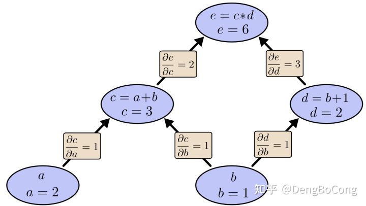
通过链式法则,我们逐节点的计算偏导数,在网络backward时,需要用链式求导法则求出网络最后输出的梯度,然后再对网络进行优化。类似上图的表达形式就是tensorflow以及pytorch的基本计算模型。总结而言,计算图模型由节点和线组成,节点表示操作符operator,或者称之为算子,线表示计算间的依赖,实线表示有数据传递依赖,传递的数据即张量,虚线通常可以表示控制依赖,即执行先后顺序。计算图从本质上说,是tensorflow在内存中构建的程序逻辑图,计算图可以被分割成多个块,并且可以并行地运行在多个不同的cpu或gpu上,这被称为并行计算。
tensorflow中的计算图有三种,分别是静态计算图,动态计算图以及autograph,tf2默认采用动态计算图,即每使用一个算子后,该算子会被动态加入到隐含的默认计算图中立即执行得到结果,每次当我们搭建完一个计算图,然后在反向传播结束之后,整个计算图就在内存中被释放了,如下示例,第二次loss.backward()就直接报错了,这也是pytorch的计算方式。动态图不区分计算图的定义和执行,定义后立即执行,称之为eager excution。
a = torch.tensor([3.0, 1.0], requires_grad=True)
b = a * a
loss = b.mean()

loss.backward() # 正常
loss.backward() # RuntimeError
较早使用静态图的方法分为两步,第一步定义计算图,第二步在会话session中执行计算图,如下是在tf1和tf2中的写法,本文用numpy实现的简单similarflow的就是这种静态图方式,静态图相比动态图是有一定效率优势的,动态图会有多次python进程和tf的c++进程之间的通信,静态图构建完成之后几乎全部再tf内核上用c++执行,效率高。
import tensorflow as tf
TensorFlow1.0
#定义计算图
g = tf.Graph()
with g.as_default():
    #placeholder为占位符,执行会话时候指定填充对象
    x = tf.placeholder(name='x', shape=[], dtype=tf.string)
    y = tf.placeholder(name='y', shape=[], dtype=tf.string)
    z = tf.string_join([x,y],name = 'join',separator=' ')
#执行计算图
with tf.Session(graph = g) as sess:
    print(sess.run(fetches = z,feed_dict = {x:"hello",y:"world"}))
tf中海油一种autograph,动态图运行效率较低,可以用@tf.function装饰器将普通python函数转换成和tf1对应的静态计算图构建代码。
2.similarflow
整体的架构是有个计算图,Graph对象,它是存储节点operation和变量的一个对象,驱动计算图是session,核心是反向传播,反向传播是通过链式求导来实现,loss对每个节点的导数之积,要实现所有的operator的导数方法,除此之外对求导有梯度下降的优化,这些是基本架构,有了这些就可以设计线性分类器,softamx以及多层感知机了。
graph设计,有向图的核心是节点,定义好节点之后放在一个图中统一管理,前向传播靠的是session。graph本身是计算图,图由节点组成,operation和variable都是节点元素,placeholder是用户输入:
class Graph(object):
    """    computational graph
"""

    def __init__(self):
        self.operations = []
        self.placeholders = []
        self.variables = []
        self.constants = []

    def __enter__(self):
        global _default_graph
        self.graph = _default_graph
        _default_graph = self
        return self

    def __exit__(self, exc_type, exc_val, exc_tb):
        global _default_graph
        _default_graph = self.graph

    def as_default(self):
        return self

class Operation(object):
    """接受一个或者更多输入节点进行简单计算
"""

    def __init__(self, *input_nodes):
        self.input_nodes = input_nodes
        self.output_nodes = []

        # 将当前节点的引用添加到输入节点的output_nodes,这样可以在输入节点中找到当前节点
        for node in input_nodes:
            node.output_nodes.append(self)

        # 将当前节点的引用添加到图中,方便后面对图中的资源进行回收等操作
        _default_graph.operations.append(self)

    def compute(self):
        """根据输入节点的值计算当前节点的输出值
"""
        pass

    def __add__(self, other):
        from .operations import add
        return add(self, other)

    def __neg__(self):
        from .operations import negative
        return negative(self)

    def __sub__(self, other):
        from .operations import add,negative
        return add(self, negative(other))

    def __mul__(self, other):
        from .operations import matmul
        return matmul(self, other)

class Placeholder(object):
    """没有输入节点,节点数据是通过图建立好以后通过用户传入
"""

    def __init__(self):
        self.output_nodes = []

        _default_graph.placeholders.append(self)

    def __add__(self, other):
        from .operations import add
        return add(self, other)

    def __neg__(self):
        from .operations import negative
        return negative(self)

    def __sub__(self, other):
        from .operations import add, negative
        return add(self, negative(other))

    def __mul__(self, other):
        from .operations import matmul
        return matmul(self, other)

class Variable(object):
    """没有输入节点,节点数据在运算过程中是可变化的
"""

    def __init__(self, initial_value=None):
        self.value = initial_value
        self.output_nodes = []

        _default_graph.variables.append(self)

    def __add__(self, other):
        from .operations import add
        return add(self, other)

    def __neg__(self):
        from .operations import negative
        return negative(self)

    def __sub__(self, other):
        from .operations import add, negative
        return add(self, negative(other))

    def __mul__(self, other):
        from .operations import matmul
        return matmul(self, other)

class Constant(object):
    """没有输入节点,节点数据在运算过程中是不可变的
"""

    def __init__(self, value=None):
        self.value = value
        self.output_nodes = []

        _default_graph.constants.append(self)

    def __add__(self, other):
        from .operations import add
        return add(self, other)

    def __neg__(self):
        from .operations import negative
        return negative(self)

    def __sub__(self, other):
        from .operations import add, negative
        return add(self, negative(other))

    def __mul__(self, other):
        from .operations import matmul
        return matmul(self, other)
1.把运算符重载一波,这样,同节点可以直接+-*了,但是由于存在相互调用,所以每次都要from import一下。
2.多用numpy代替python自己的运算。
session:feedforward:需要一个session来对一个已经创建好的计算图进行计算,已创建的graph的节点其实只是创建了一个空节点,节点中并没有可以计算的数值,session先递归后序遍历拿到operation前的所有节点,调用节点的compute方法得到值。
import numpy as np
from .graph import Operation, Placeholder, Variable, Constant

class Session(object):
    """ feedforward
"""

    def __init__(self):
        self.graph = _default_graph

    def __enter__(self):
        return self

    def __exit__(self, exc_type, exc_val, exc_tb):
        return self.close()

    def close(self):
        all_nodes = (self.graph.operations + self.graph.variables +
                     self.graph.constants + self.graph.placeholders)
        for node in all_nodes:
            node.output = None

    def run(self, operation, feed_dict=None):
        """   计算节点的输出值
        :param operation:
        :param feed_dict:
        :return:
"""
        nodes_postorder = traverse_postorder(operation)

        for node in nodes_postorder:
            if type(node) == Placeholder:
                node.output = feed_dict[node]
            elif (type(node) == Variable) or (type(node) == Constant):
                node.output = node.value
            else:  # Operation
                # 取出每个节点的值
                node.inputs = [input_node.output for input_node in node.input_nodes]
                # 拆包,调用operation的compute计算前向值
                node.output = node.compute(*node.inputs)

            if type(node.output) == list:
                node.output = np.array(node.output)
        return operation.output

def traverse_postorder(operation):
"""
    通过后序遍历获取一个节点所需的所有节点的输出值,递归
    :param operation:
    :return:
"""
    nodes_postorder = []

    def recurse(node):
        if isinstance(node, Operation):
            for input_node in node.input_nodes:
                recurse(input_node)
        nodes_postorder.append(node)

    recurse(operation)
    return nodes_postorder
operation:算子中只实现了前向方法,反向传播的梯度计算放在单独的文件中。
import numpy as np
from .graph import Operation

class matmul(Operation):
    def __init__(self, x, y):
        super(matmul, self).__init__(x, y)

    def compute(self, x_value, y_value):
        """ x_value,y_value是具体的值,而非节点中的类型,如果直接用self.input_nodes就是garph中的节点,
        init和compute都传参确实看起来很丑,==!
        :param x_value:
        :param y_value:
        :return:
"""
        return np.dot(x_value, y_value)

class add(Operation):
    def __init__(self, x, y):
        super(add, self).__init__(x, y)

    def compute(self, x_value, y_value):
        return np.add(x_value, y_value)

class negative(Operation):
    def __init__(self, x):
        super(negative, self).__init__(x)

    def compute(self, x_value):
        return -x_value

class multiply(Operation):
    def __init__(self, x, y):
        super(multiply, self).__init__(x, y)

    def compute(self, x_value, y_value):
        return np.multiply(x_value, y_value)

class sigmoid(Operation):
    def __init__(self, x):
        super(sigmoid, self).__init__(x)

    def compute(self, x_value):
        return 1 / (1 + np.exp(-x_value))

class softmax(Operation):
    def __init__(self, x):
        super(softmax, self).__init__(x)

    def compute(self, x_value):
        return np.exp(x_value) / np.sum(np.exp(x_value), axis=1)[:, None]

class log(Operation):
    def __init__(self, x):
        super(log, self).__init__(x)

    def compute(self, x_value):
        return np.log(x_value)

class square(Operation):
    def __init__(self, x):
        super(square, self).__init__(x)

    def compute(self, x_value):
        return np.square(x_value)

class reduce_sum(Operation):
    def __init__(self, A, axis=None):
        super(reduce_sum, self).__init__(A)
        self.axis = axis

    def compute(self, A_value):
        return np.sum(A_value, self.axis)
gradients:梯度计算
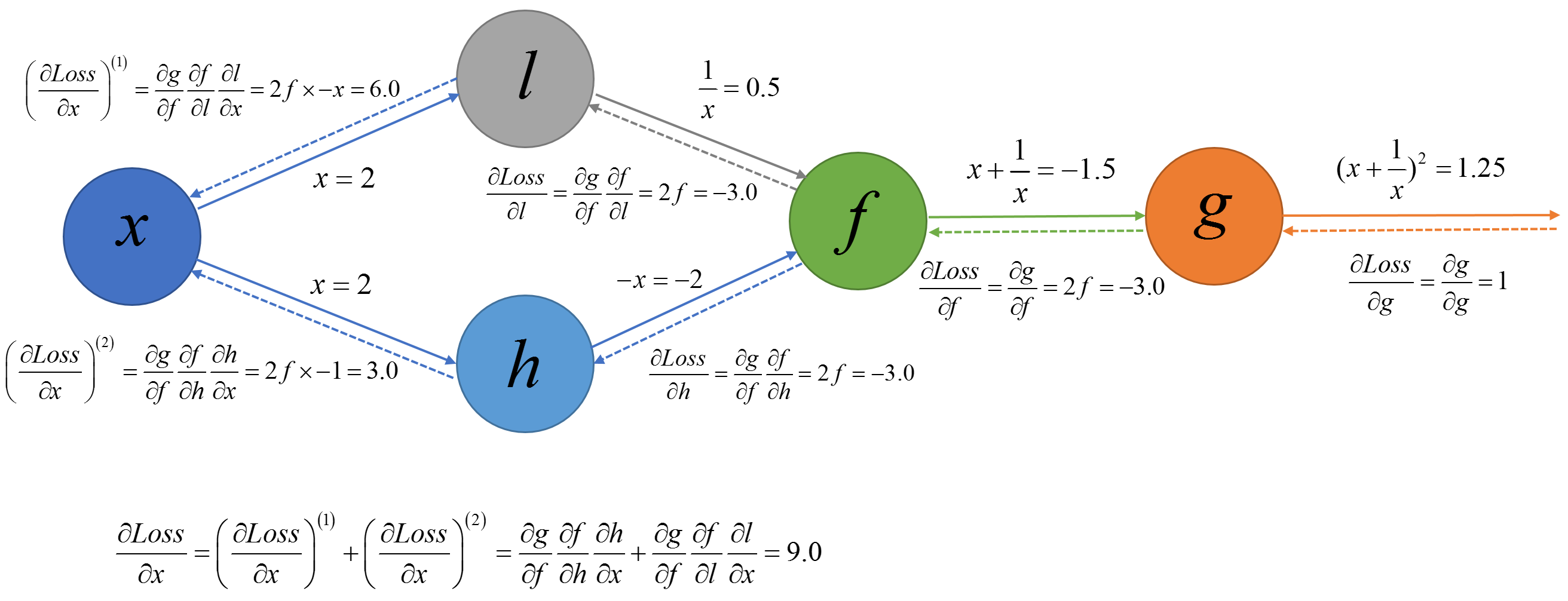
反向传播,矩阵梯度的计算是实现反向传播算法重要的一部分。在网络中基本都是求矩阵对矩阵的导数,不要直接计算一个矩阵对另一个矩阵的导数,可以利用loss这个标量做间接的维度求导,确定了维度,就好算梯度了。
算子求导数这块softmax要关注,另外用了注册器,后面在反向传播中直接用op_type在字典中调。
import numpy as np

_gradient_registry = {}

class RegisterGradient(object):
    def __init__(self, op_type):
        self._op_type = eval(op_type)

    def __call__(self, f):
        _gradient_registry[self._op_type] = f
        return f

@RegisterGradient("add")
def _add_gradient(op, grad):
    """   求和矩阵求导,行相加,列相加
    :param op:
    :param grad:
    :return:
"""
    x, y = op.inputs[0], op.inputs[1]

    grad_wrt_x = grad
    while np.ndim(grad_wrt_x) > len(np.shape(x)):
        grad_wrt_x = np.sum(grad_wrt_x, axis=0)
    for axis, size in enumerate(np.shape(x)):
        if size == 1:
            grad_wrt_x = np.sum(grad_wrt_x, axis=axis, keepdims=True)

    grad_wrt_y = grad
    while np.ndim(grad_wrt_y) > len(np.shape(y)):
        grad_wrt_y = np.sum(grad_wrt_y, axis=0)
    for axis, size in enumerate(np.shape(y)):
        if size == 1:
            grad_wrt_y = np.sum(grad_wrt_y, axis=axis, keepdims=True)

    return [grad_wrt_x, grad_wrt_y]

@RegisterGradient("matmul")
def _matmul_gradient(op, grad):
    """ 求x的梯度:y的转置,求y的梯度:x的转置
    :param op:
    :param grad:
    :return:
"""
    x, y = op.inputs[0], op.inputs[1]
    return [np.dot(grad, np.transpose(y)), np.dot(np.transpose(x), grad)]

@RegisterGradient("sigmoid")
def _sigmoid_gradient(op, grad):
    sigmoid = op.output
    return grad * sigmoid * (1 - sigmoid)

@RegisterGradient("softmax")
def _softmax_gradient(op, grad):
    """ softmax 倒数
    https://stackoverflow.com/questions/40575841/numpy-calculate-the-derivative-of-the-softmax-function
    :param op:
    :param grad:
    :return:
"""
    softmax = op.output
    return (grad - np.reshape(np.sum(grad * softmax, 1), [-1, 1])) * softmax

@RegisterGradient("log")
def _log_gradient(op, grad):
    x = op.inputs[0]
    return grad / x

@RegisterGradient("multiply")
def _multiply_gradient(op, grad):
    x, y = op.inputs[0], op.inputs[1]
    return [grad * y, grad * x]

@RegisterGradient("negative")
def _negative_gradient(op, grad):
    return -grad

@RegisterGradient("square")
def _square_gradient(op, grad):
    x = op.inputs[0]
    return grad * np.multiply(2.0, x)

@RegisterGradient("reduce_sum")
def _reduce_sum_gradient(op, grad):
    x = op.inputs[0]

    output_shape = np.array(np.shape(x))
    output_shape[op.axis] = 1
    tile_scaling = np.shape(x) // output_shape
    grad = np.reshape(grad, output_shape)
    return np.tile(grad, tile_scaling)
反向传播:
import numpy as np
from queue import Queue

from .graph import Operation, Variable
from .gradients import _gradient_registry

def compute_gradients(loss):
    """ 已知每个节点中输出对输入的梯度,从后往前反向搜索与损失节点相关联的节点进行反向传播计算梯度。
    若我们需要计算其他节点关于loss的梯度需要以损失节点为启动对计算图进行广度优先搜索,在搜索过程中
    针对每个节点的梯度计算便可以一边遍历一边计算计算节点对遍历节点的梯度,可以用dict将节点与梯度进行保存。

    使用一个先进先出的队列控制遍历顺序,一个集合对象存储已访问的节点防止重复访问,然后遍历的时候计算梯度并将
    梯度放到grad_table中
    :param loss:
    :return:
"""
    grad_table = {}  # 存放节点的梯度
    grad_table[loss] = 1

    visited = set()
    queue = Queue()
    visited.add(loss)
    queue.put(loss)

    while not queue.empty():
        node = queue.get()

        # 该节点不是loss节点,先遍历进queue
        if node != loss:
            grad_table[node] = 0

            for output_node in node.output_nodes:
                lossgrad_wrt_output_node_output = grad_table[output_node]

                output_node_op_type = output_node.__class__
                bprop = _gradient_registry[output_node_op_type]

                lossgrads_wrt_output_node_inputs = bprop(output_node, lossgrad_wrt_output_node_output)

                if len(output_node.input_nodes) == 1:
                    grad_table[node] += lossgrads_wrt_output_node_inputs
                else:
                    # 若一个节点有多个输出,则多个梯度求和
                    node_index_in_output_node_inputs = output_node.input_nodes.index(node)
                    lossgrad_wrt_node = lossgrads_wrt_output_node_inputs[node_index_in_output_node_inputs]
                    grad_table[node] += lossgrad_wrt_node

        # 把节点存入到队列中
        if hasattr(node, "input_nodes"):
            for input_node in node.input_nodes:
                if input_node not in visited:
                    visited.add(input_node)
                    queue.put(input_node)

    return grad_table
GradientDescentOptimizer:梯度下降优化,实现了损失函数对其他节点梯度的计算,得到梯度的目的是为了能够优化参数,实现了一个梯度下降优化器来完成参数优化,以梯度的反方向作为每轮迭代的搜索方向然后根据设定的步长对局部最优值进行搜索:
class GradientDescentOptimizer(object):
    def __init__(self, learning_rate):
        self.learning_rate = learning_rate

    def minimize(self, loss):
        learning_rate = self.learning_rate

        class MinimizationOperation(Operation):
            def compute(self):
                grad_table = compute_gradients(loss)

                for node in grad_table:
                    if type(node) == Variable or type(node) == Constant:
                        grad = grad_table[node]
                        node.value -= learning_rate * grad

        return MinimizationOperation()
举个例子:线性分类
import numpy as np
import matplotlib.pylab as plt
import similarflow as sf

input_x = np.linspace(-1, 1, 100)
input_y = input_x * 3 + np.random.randn(input_x.shape[0]) * 0.5

x = sf.Placeholder()
y = sf.Placeholder()
w = sf.Variable([[1.0]])
b = sf.Variable(0.0)

linear = sf.add(sf.matmul(x, w), b)
linear = x * w + b

loss = sf.reduce_sum(sf.square(sf.add(linear, sf.negative(y))))
loss = sf.reduce_sum(sf.square(linear - y))

train_op = sf.train.GradientDescentOptimizer(learning_rate=0.005).minimize(loss)

feed_dict = {x: np.reshape(input_x, (-1, 1)), y: np.reshape(input_y, (-1, 1))}
feed_dict = {x: input_x, y: input_y}

with sf.Session() as sess:
    for step in range(20):
        # 前向
        loss_value = sess.run(loss, feed_dict)
        mse = loss_value / len(input_x)
        print(f"step:{step},loss:{loss_value},mse:{mse}")
        # 反向传播
        sess.run(train_op, feed_dict)
    w_value = sess.run(w, feed_dict=feed_dict)
    b_value = sess.run(b, feed_dict=feed_dict)
    print(f"w:{w_value},b:{b_value}")

w_value = float(w_value)
max_x, min_x = np.max(input_x), np.min(input_x)
max_y, min_y = w_value * max_x + b_value, w_value * min_x + b_value

plt.plot([max_x, min_x], [max_y, min_y], color='r')
plt.scatter(input_x, input_y)
plt.show()
感知机:
import numpy as np
import similarflow as sf
import matplotlib.pyplot as plt

Create red points centered at (-2, -2)
red_points = np.random.randn(50, 2) - 2 * np.ones((50, 2))

Create blue points centered at (2, 2)
blue_points = np.random.randn(50, 2) + 2 * np.ones((50, 2))

X = sf.Placeholder()
y = sf.Placeholder()
W = sf.Variable(np.random.randn(2, 2))
b = sf.Variable(np.random.randn(2))

p = sf.softmax(sf.add(sf.matmul(X, W), b))

loss = sf.negative(sf.reduce_sum(sf.reduce_sum(sf.multiply(y, sf.log(p)), axis=1)))

train_op = sf.train.GradientDescentOptimizer(learning_rate=0.01).minimize(loss)

feed_dict = {
    X: np.concatenate((blue_points, red_points)),
    y: [[1, 0]] * len(blue_points) + [[0, 1]] * len(red_points)
}

with sf.Session() as sess:
    for step in range(100):
        loss_value = sess.run(loss, feed_dict)
        if step % 10 == 0:
            print(f"step:{step},loss:{loss_value}")
        sess.run(train_op, feed_dict)

    # Print final result
    W_value = sess.run(W)
    print("Weight matrix:\n", W_value)
    b_value = sess.run(b)
    print("Bias:\n", b_value)

Plot a line y = -x
x_axis = np.linspace(-4, 4, 100)
y_axis = -W_value[0][0] / W_value[1][0] * x_axis - b_value[0] / W_value[1][0]
plt.plot(x_axis, y_axis)

Add the red and blue points
plt.scatter(red_points[:, 0], red_points[:, 1], color='red')
plt.scatter(blue_points[:, 0], blue_points[:, 1], color='blue')
plt.show()
多层感知机
import numpy as np
import similarflow as sf
import matplotlib.pyplot as plt

Create two clusters of red points centered at (0, 0) and (1, 1), respectively.

red_points = np.concatenate((
    0.2 * np.random.randn(25, 2) + np.array([[0, 0]] * 25),
    0.2 * np.random.randn(25, 2) + np.array([[1, 1]] * 25)
))

Create two clusters of blue points centered at (0, 1) and (1, 0), respectively.

blue_points = np.concatenate((
    0.2 * np.random.randn(25, 2) + np.array([[0, 1]] * 25),
    0.2 * np.random.randn(25, 2) + np.array([[1, 0]] * 25)
))

Plot them
plt.scatter(red_points[:, 0], red_points[:, 1], color='red')
plt.scatter(blue_points[:, 0], blue_points[:, 1], color='blue')
plt.show()

X = sf.Placeholder()
y = sf.Placeholder()
W_hidden = sf.Variable(np.random.randn(2, 2))
b_hidden = sf.Variable(np.random.randn(2))
p_hidden = sf.sigmoid(sf.add(sf.matmul(X, W_hidden), b_hidden))

W_output = sf.Variable(np.random.randn(2, 2))
b_output = sf.Variable(np.random.rand(2))
p_output = sf.softmax(sf.add(sf.matmul(p_hidden, W_output), b_output))

loss = sf.negative(sf.reduce_sum(sf.reduce_sum(sf.multiply(y, sf.log(p_output)), axis=1)))

train_op = sf.train.GradientDescentOptimizer(learning_rate=0.03).minimize(loss)

feed_dict = {
    X: np.concatenate((blue_points, red_points)),
    y: [[1, 0]] * len(blue_points) + [[0, 1]] * len(red_points)
}

with sf.Session() as sess:
    for step in range(100):
        loss_value = sess.run(loss, feed_dict)
        if step % 10 == 0:
            print(f"step:{step},loss:{loss_value}")
        sess.run(train_op, feed_dict)

    # Print final result
    W_hidden_value = sess.run(W_hidden)
    print("Hidden layer weight matrix:\n", W_hidden_value)
    b_hidden_value = sess.run(b_hidden)
    print("Hidden layer bias:\n", b_hidden_value)
    W_output_value = sess.run(W_output)
    print("Output layer weight matrix:\n", W_output_value)
    b_output_value = sess.run(b_output)
    print("Output layer bias:\n", b_output_value)

Visualize classification boundary
xs = np.linspace(-2, 2)
ys = np.linspace(-2, 2)
pred_classes = []
for x in xs:
    for y in ys:
        pred_class = sess.run(p_output, feed_dict={X: [[x, y]]})[0]
        pred_classes.append((x, y, pred_class.argmax()))
xs_p, ys_p = [], []
xs_n, ys_n = [], []
for x, y, c in pred_classes:
    if c == 0:
        xs_n.append(x)
        ys_n.append(y)
    else:
        xs_p.append(x)
        ys_p.append(y)
plt.plot(xs_p, ys_p, 'ro', xs_n, ys_n, 'bo')
plt.show()
Original: https://blog.csdn.net/u012193416/article/details/122958900
Author: Kun Li
Title: 用numpy实现tensorflow式的深度学习框架similarflow
原创文章受到原创版权保护。转载请注明出处:https://www.johngo689.com/511196/
转载文章受原作者版权保护。转载请注明原作者出处!