

该文章适合OpenCv的初学者以及对计算机视觉有了简单认识的朋友。以下将根据不同的能力水平进行梯度的讲解。最后会附带完整代码。
小白需要知道的
什么是传统的视觉寻迹?
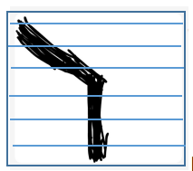
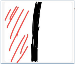
在我看来,传统的跟踪是通过记录轨迹的横坐标来判断的。例如:
[En]
In my opinion, the traditional tracking is judged by recording the Abscissa of the track. For example:
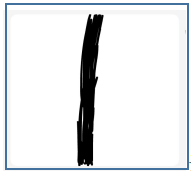

这幅画被认为是笔直的。但机器怎么能判断呢?
[En]
This picture is considered to be straight. But how can the machine judge?
我们可以通过将图片转换成矩阵来判断,然后通过记录这些黑点的所有时间的横坐标来判断,从而得到黑点的平均横坐标。
[En]
We can judge by converting the picture into a matrix, and then by recording the Abscissa of these black dots all the time, so as to obtain the average Abscissa of the black dot.
source = 0  # 记录黑点的横坐标
m = 0  # 记录黑点个数
y = 143  # 画面的横轴大小
x = 80  # 画面的纵轴大小
for i in range(y):
    for j in range(x):
        if pred[j, i] == 0:
            m += 1
            source += j
source /= m  # 获得平均横坐标
source -= x / 2  # 对比中轴差值
if abs(source)  0:
    print("左转")
else:
    print("右转")
上面代码pred为画面的矩阵。当平均横坐标与x中轴值大小偏差10以内就被认为”直行”。
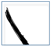
同样,根据平均水平坐标值的计算,这两张图片被视为“左转”,机器被很好地识别出来。
[En]
By the same token, according to the calculation of the average horizontal coordinate value, the two pictures are regarded as “turning left” and the machine is well identified.
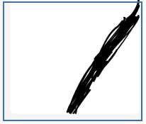
这是一样的事情,这被机器认为是右转。
[En]
It’s the same thing, which is regarded as a right turn by the machine.
寻迹的思想
通过上面的简要介绍,我们对机器对轨迹的简单识别有了很好的了解。它也是一种传统的视觉方法。
[En]
From the above brief introduction, we have a good understanding of the simple recognition of the machine for the trajectory. It is also a traditional visual method.
接下来,我们将介绍跟踪的想法。
[En]
Next, we will introduce the idea of tracking.
有朋友可能会问:上面的图片都是黑白的,轨迹是黑色的,不符合实际。那么我们需要怎么做呢?
[En]
A friend may ask: the above pictures are all black and white, and the track is black, which is not consistent with reality. So how do we need to do this?
总的来说分为:获取图片(RGB) —> 转为灰度图 —–> 转为二值图 —-> 转为矩阵
THRESHOLD = 80 # 设置阈值为80
ret, frame = capture.read()  # 一帧一帧读取视频
gray = cv.cvtColor(frame, cv.COLOR_BGR2GRAY)  # 对每一帧做处理,设置为灰度图
retval, black_Write = cv.threshold(gray, THRESHOLD, 255, cv.THRESH_BINARY)  # 将灰度图二值化
data = np.array(black_Write)  # 把这个数据通过 numpy 转换成多维度的张量
在转化为灰度图的时候,会将RGB三颜色通道转换为0~255的灰度图,0表示纯黑,255表示纯白。
转化为二值图的先决条件就是要转换为灰度图,然后通过设置阈值将灰度图所有的像素点分割为0和255两种颜色。上述代码第三行的THRESHOULD是就是阈值,大小在0~255之间。我这里设置的就是80。
进阶知识
矩阵的处理—缩小矩阵
最开始测试的时候,我用的是10块钱二手买来的USB免驱摄像头。拍摄分辨率为640*480,在遍历时我们大多数会选择二重for循环进行,然后进行判断。但是这是十分消耗时间的。因此对于矩阵的处理显得尤为重要。接下来将介绍方法一:缩小矩阵。
X_LEFT_CUT_NUM = 199
X_RIGHT_CUT_NUM = 439
Y_HIGH_CUT_NUM = 439
Y_LOW_CUT_NUM = 239
data_after = data[X_LEFT_CUT_NUM:X_RIGHT_CUT_NUM, Y_LOW_CUT_NUM:Y_HIGH_CUT_NUM]  # 裁剪图像,获得一个200*240
data为经过二值化后得到的矩阵。
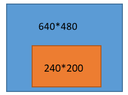
你通过种植得到的是橙色区域。对于车辆的跟踪,正好这块区域是最需要关注的,离车很近,是下一步会到达的区域。与遍历480到640的矩阵相比,遍历该矩阵的时间大大减少。
[En]
What you get by cropping is the orange area. For the car tracking, just this area is the most need for concern, very close to the car, is the next step will arrive in the area. Compared to traversing a matrix of 480 to 640, the time to traverse this matrix is greatly reduced.
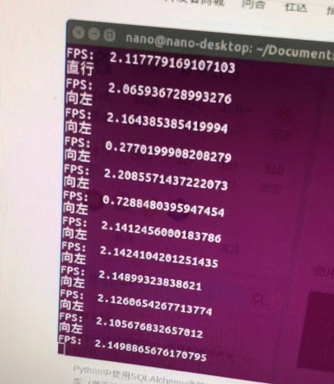
但是,依旧非常的消耗时间,我的测试平台是NVIDIA Jetson nano,得到的帧数竟然只有2帧。对于这块板子来说是非常不理想的,于是就分析了原因。nano这块板子强于树莓派就在于它具有128个CUDA,处理图像以及做流式计算会大幅度加快。但是因为还没有用到张量的运算,因此这里还是取决于CPU的处理速度。
在我添加了时间戳之后,一切都变得清晰起来,而且遍历矩阵的速度太慢了。
[En]
Everything became clear after I added the timestamp, and the traversal of the matrix was too slow.
平均采样
对于上述问题,我可以想到一个解决方案,平均抽样。当我们处理一张图片时,我们真的不需要判断每一行。例如,现在我需要遍历200行,而我只需要遍历其中的20行就可以得到这个趋势。
[En]
For the above problems, I can think of a solution, average sampling. We don’t really need to judge each line when we deal with a picture. For example, now I need to traverse 200 rows, and I only need to traverse 20 of them to get this trend.
source = 0  # 记录黑点的横坐标
m = 0  # 记录黑点个数
y = int(200 / 20)  # 画面的纵轴大小
x = 240  # 画面的横轴大小
for i in range(y):
    for j in range(x):
        if pred[j, i * 10] == 0:
            m += 1
            source += j
这里我选择了每20行取一行,果然帧数上升了。成功到了八帧。。。
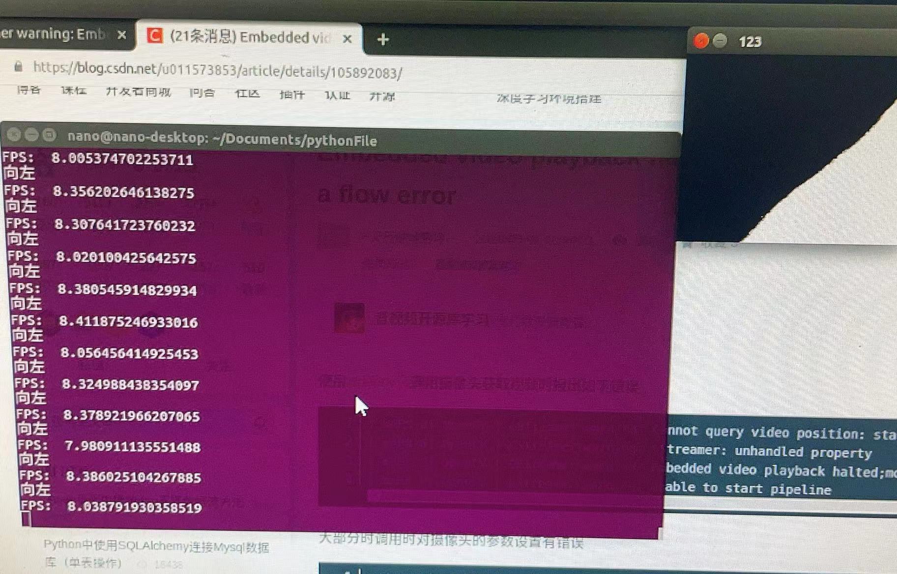
右边的窗口是图像。但仅仅寻找痕迹是不够的。现在我们已经到了矩阵的末尾,我们必须考虑其他方法。
[En]
The window on the right is the image. But it’s not enough to look for traces. Now that we’ve come to the end of the matrix, we have to think of other ways.
池化操作
前面有谈到,到目前为止,因为没有使用矩阵的运算,因此没有发挥出NVIDIA Jetson nano这块开发板的优势,所以我们可以想想如何往这方面靠靠。碰巧我今年暑假接触过一点计算机视觉的网上课程。我就想到了池化的操作。
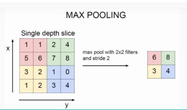
池化操作分为最大池化和平均池化。如上图所示,其核心是用卷积核来缩小图像的尺寸,并用局部特征来代替整体的一种–中国方法。最大池操作的操作速度会更快,但会丢失一些细节。平均池化是基于卷积内核中所有值的平均值,而不是整个值,因此操作会稍微慢一些,但细节将被保留。
[En]
Pooling operations are divided into maximum pooling and average pooling. As shown in the above figure, the core is to use convolution cores to reduce the size of the image and use local features to replace the overall one-China approach. The operation speed of the maximum pooling operation will be faster, but some details will be lost. The average pooling is based on the average of all the values in the convolution kernel instead of the whole, so the operation will be a little slower, but the details will be retained.
拼合运算不同于卷积运算,拼合卷积核可以看作是具有相同权值的卷积。池化只会减小图片的大小并转换尺寸。如果我们走得太远,我们在这里只使用池化方法。要理解意思,你只需要知道这是一种使用局部特征而不是整体特征的方式,这可以缩小画面的大小,但也可以很好地代表画面。
[En]
Pooling operation is different from convolution, pooled convolution kernel can be regarded as convolution with the same weight. Pooling only reduces the size of the picture and converts the dimensions. If we go too far, we only use the pooling method here. To understand the meaning, you just need to know that it is a way to use local features instead of the whole, which can reduce the size of the picture, but it can also represent the picture very well.
STRIDE = 3  # 步数
data_after = tf.convert_to_tensor(data, tf.float32, name='data_after')
data_after = tf.expand_dims(data_after, axis=0)  # 拓展为三维张量
data_after = tf.expand_dims(data_after, axis=3)  # 拓展为三维张量
out = tf.nn.avg_pool(data_after, [1, STRIDE, STRIDE, 1], [1, STRIDE, STRIDE, 1], 'SAME')  # 平均池化,后面的数组为跳转步数
data_after为上面经过二值化得到的矩阵。shape为[240,200]但是进行池化操作需要进行维度扩展,否则无法使用卷积核进行池化操作。进行了第3、4行的操作后shape为[1,240,200,1]。就可以进行池化操作了。
池化操作的第1个参数需要处理的矩阵;
第2个参数为卷积核,数组的第一个和最后一个为必须为1,中间两个数表示卷积核大小,例如这里就是3*3的卷积核;
第3个参数为移动的步长,卷积核在图像上移动才能得到处理后的图像。与上面一样数组里第1个和最后一个为1,表示会遍历所有的维度,中间两个数为横向移动和纵向移动的步长。
第四个参数选择为”VALID”和”SAME”分别表示为是否需要边界填充。对于新手来说,如果搞不清楚直接选择”SAME”方便计算池化后的大小。
通过上述操作,我使用3*3的卷积核,步长为3进行池化操作得到的处理后的图片x轴缩小了3倍,y轴缩小了3倍。平均取样间隔该到了10行一次,此时我在运行时,以及达到了30帧+了。(其实以及达到了上限,后来我将平均采样该到了5行一次,依然能保持24帧+)
算法优化(重点)
240200的矩阵卷积之后变成了8067的矩阵,由于每10行取样一次,就可能造成得到的值不能很好的表现当前的情况。因此我们需要想办法优化算法。
二次池化
前面提到,80-67的矩阵是通过收割和拼接获得的,接受视野很窄,不能用来判断稍远一点的情况。最直观的变化是,车速不可能很快,一旦速度超过前一帧,那么视觉跟踪就变得毫无意义。
[En]
It is mentioned earlier that the matrix of 80mm 67 is obtained by cropping and pooling, and the receptive field is very narrow and can not be used to judge the situation a little further away. The most intuitive change is that the speed of the car can not be very fast, once the speed exceeds the previous frame, then visual tracking will become meaningless.
在此,就提出了二次池化,用池化代替裁剪。就可以获得了更大的感受野。此时我也将摄像头改为了板载摄像头。以下是板载摄像头的打开方式,CSI摄像头用ViserCapture是无法打开的,需要进行配置。
def gstreamer_pipeline(
        capture_width=1280,
        capture_height=720,
        display_width=1280,
        display_height=720,
        framerate=60,
        flip_method=0,
):
    return (
            "nvarguscamerasrc ! "
            "video/x-raw(memory:NVMM), "
            "width=(int)%d, height=(int)%d, "
            "format=(string)NV12, framerate=(fraction)%d/1 ! "
            "nvvidconv flip-method=%d ! "
            "video/x-raw, width=(int)%d, height=(int)%d, format=(string)BGRx ! "
            "videoconvert ! "
            "video/x-raw, format=(string)BGR ! appsink"
            % (
                capture_width,
                capture_height,
                framerate,
                flip_method,
                display_width,
                display_height,
            )
    )

capture = cv.VideoCapture(gstreamer_pipeline(flip_method=0), cv.CAP_GSTREAMER)  # 创建一个VideoCapture对象
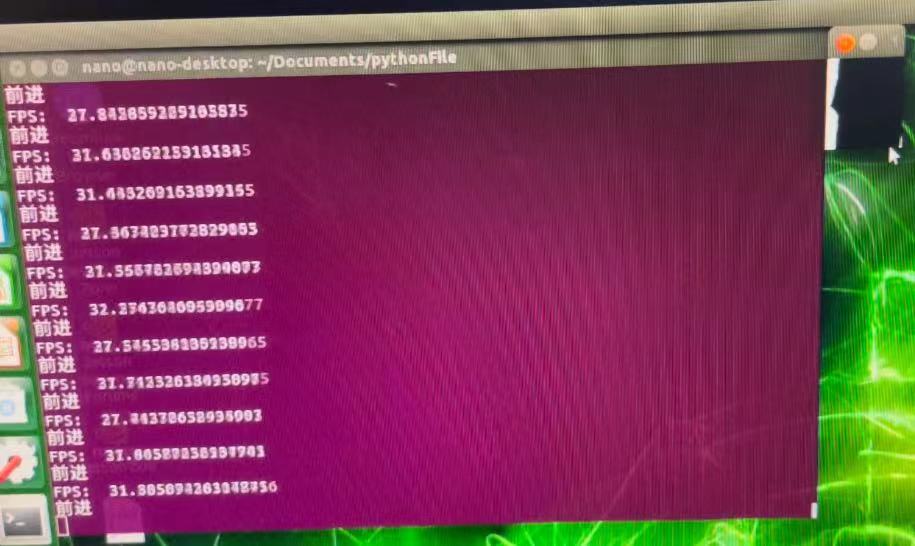
此时窗口大小变为了1280720,进行了两次33卷积核,步长为3的池化操作,窗口大小变为了142*80,平均采样为10行采样一行。
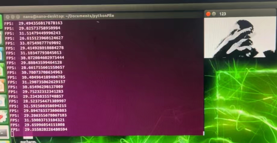
当时我在动,可以看到感觉场很大,在这么复杂的环境下还能保持在30帧左右。(后来,当平均采样为每行5行时,帧的数量保持在24帧左右。)到目前为止,画面的接受场和表达都做得很好。
[En]
At that time, I was moving, and I could see that the sensory field was very large, and it could still be maintained at about 30 frames in such a complex environment. (later, when the average sampling was 5 lines per row, the number of frames was maintained at around 24 frames.) so far, the receptive field and the expression of the picture have been done well.
有的朋友会问,为什么要经过两次池化,而不是一次池化原则更大的卷积核以及步长呢?回答这个问题,首先卷积核池化一次只会输出一个值即一个特征,那么就意味着在该值下的其他特征就会被覆盖。大的卷积核得到的图片就不会有二次卷积得到的图片包含的特征细腻。其次,著名AlexNet在当年的人工智能大赛获得冠军就证明了连续多个小型卷积核的组合效果优于大型卷积核。
判断优化
对于”直行”来说左侧空白处,是不需要判断的,进行判断十分浪费时间,并且没有意义。
同理对于”右转”来说亦是如此。
然后,您可以通过上一次图像处理获得的命令来选择当前图像的处理范围。它很好地解决了上述问题。
[En]
Then you can select the processing range of the current image through the command obtained from the previous image processing. It solves the problems mentioned above very well.
然后我们再想,赛道右侧的空白部分是不是也没有必要去判断呢?
[En]
Then we think again, whether the blank part on the right side of the track is also unnecessary to judge?
在这里,我设计了一个算法,当扫描矩阵的每一行时,得到轨迹后,如果连续有多个白点,则直接跳出当前循环。
[En]
Here I have designed an algorithm, when scanning each row of the matrix, after getting the trajectory, if there are multiple white dots in succession, then directly jump out of the current loop.
STRIDE = 3
CAPTURE_WIDTH = 1280  # 摄像头捕捉画面宽
CAPTURE_HEIGHT = 720  # 摄像头捕捉画面高
order = ""  # 保存上一条指令
RANGE_NUM = 10  # 直行允许波动范围
while True:
    source = 0  # 记录黑点的横坐标
    black_point_num = 0  # 代表黑点个数
    x = int(CAPTURE_WIDTH / STRIDE / STRIDE)
    y = int(CAPTURE_HEIGHT / STRIDE / STRIDE)
    opt = 0
    if order == "前进":
        opt = int(x / 4)
    elif order == "右转":
        opt = int(x / 3)
    else:
        opt = 0
    for i in range(y):
        row = 0  # 记录当前行的黑点数量
        row_white_point_num = 0  # 代表行白点个数
        for j in range(opt, x):
            if pred[i, j] == 0:
                row += 1
                row_white_point_num = 0
                source += j
            else:
                row_white_point_num += 1
                if row > 5 and row_white_point_num > 5:
                    break
        black_point_num += row
    source /= black_point_num  # 获得平均横坐标
    source -= x / 2
    if abs(source)  0:
        print("右转")
        order = "右转"
    else:
        print("左转")
        order = "左转"
为了验证这种效率,我取消了平均抽样。目前的情况是遍历142-80的矩阵。
[En]
To verify this efficiency, I canceled the average sampling. The current condition is to traverse the matrix of 142-80.
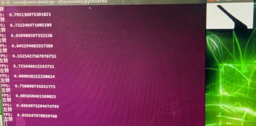
在没有判断和优化的情况下,可以看到帧的数量在6.5帧左右。
[En]
Without judgment and optimization, you can see that the number of frames is about 6.5.
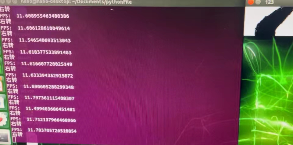
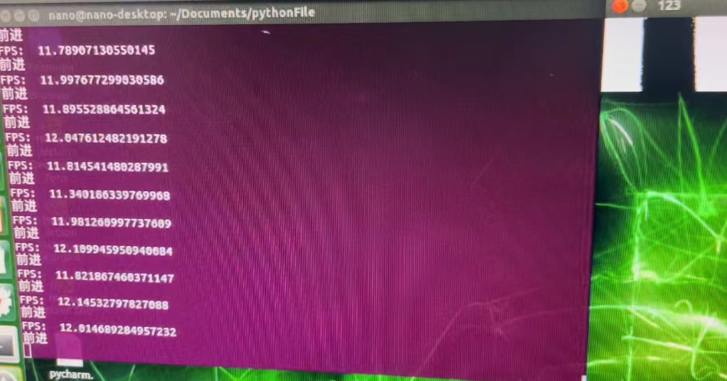
经过优化判断,帧数在12帧左右,效率几乎翻了一番。
[En]
After the optimization judgment, the number of frames is about 12 frames, and the efficiency is almost doubled.
完整代码
优化前
开发作者 :Tian.Z.L
开发时间 :2022/1/9 21:33
文件名称 :vision.PY
开发工具 :PyCharm
import time
import Adafruit_SSD1306
import cv2 as cv
import numpy as np
import tensorflow as tf
from PIL import Image
THRESHOLD = 100 # 二值化阈值
STRIDE = 3
X_LEFT_CUT_NUM = 199
X_RIGHT_CUT_NUM = 439
Y_HIGH_CUT_NUM = 439
Y_LOW_CUT_NUM = 239
RANGE_NUM = 10
注意 使用的是哪组i2c的接口,对应调整i2c_bus取值
OLED = Adafruit_SSD1306.SSD1306_128_64(rst=None, i2c_bus=1, gpio=1)
OLED.begin() # 初始化屏幕并清屏
OLED.clear()
OLED.display()
def gstreamer_pipeline(
capture_width=1280,
capture_height=720,
display_width=1280,
display_height=720,
framerate=60,
flip_method=0,
):
return (
"nvarguscamerasrc ! "
"video/x-raw(memory:NVMM), "
"width=(int)%d, height=(int)%d, "
"format=(string)NV12, framerate=(fraction)%d/1 ! "
"nvvidconv flip-method=%d ! "
"video/x-raw, width=(int)%d, height=(int)%d, format=(string)BGRx ! "
"videoconvert ! "
"video/x-raw, format=(string)BGR ! appsink"
% (
capture_width,
capture_height,
framerate,
flip_method,
display_width,
display_height,
)
)
capture = cv.VideoCapture(gstreamer_pipeline(flip_method=0), cv.CAP_GSTREAMER) # 创建一个VideoCapture对象
start_time = time.time()
while (True):
ret, frame = capture.read() # 一帧一帧读取视频
gray = cv.cvtColor(frame, cv.COLOR_BGR2GRAY) # 对每一帧做处理,设置为灰度图
retval, black_Write = cv.threshold(gray, THRESHOLD, 255, cv.THRESH_BINARY) # 将灰度图二值化
data = np.array(black_Write) # 把这个数据通过 numpy 转换成多维度的张量
# data_after = data[X_LEFT_CUT_NUM:X_RIGHT_CUT_NUM, Y_LOW_CUT_NUM:Y_HIGH_CUT_NUM] # 裁剪图像,获得一个200*240
data_after = tf.convert_to_tensor(data, tf.float32, name='data_after')
data_after = tf.expand_dims(data_after, axis=0) # 拓展为三维张量
data_after = tf.expand_dims(data_after, axis=3) # 拓展为三维张量
# out = tf.nn.avg_pool(data_after, [1, STRIDE, STRIDE, 1], [1, STRIDE, STRIDE, 1], 'SAME') # 平均池化,后面的数组为跳转步数
out = tf.nn.max_pool(data_after, [1, STRIDE, STRIDE, 1], [1, STRIDE, STRIDE, 1], 'SAME') # 最大池化,后面的数组为跳转步数
out = tf.nn.max_pool(out, [1, STRIDE, STRIDE, 1], [1, STRIDE, STRIDE, 1], 'SAME')
# print(out)
out = tf.squeeze(out) # 缩小张量维度,将所有维度为1的去除掉,在这里就表现只剩下二值图
pred = np.array(out, np.uint8)
cv.imshow('123', pred) # 显示结果
source = 0 # 记录黑点的横坐标
m = 0 # 记录黑点个数
y = 143 # 画面的横轴大小
x = 80 # 画面的纵轴大小
for i in range(y):
for j in range(x):
if pred[j, i] == 0:
m += 1
source += j
if cv.waitKey(1) & 0xFF == ord('q'): # 按q停止
break
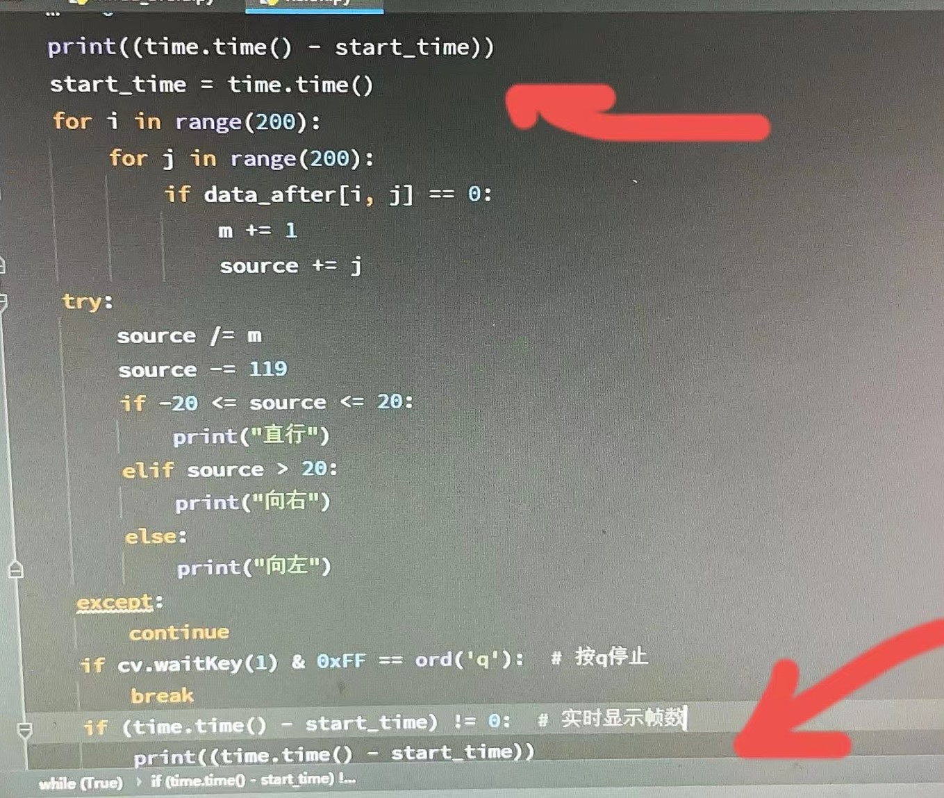
if (time.time() - start_time) != 0: # 实时显示帧数
# print((time.time() - start_time))
print("FPS: ", 1 / (time.time() - start_time))
try:
source /= m # 获得平均横坐标
source -= x / 2
if abs(source) <= 10: print("前进") elif source> 0:
print("左转")
else:
print("右转")
start_time = time.time()
except:
start_time = time.time()
print("停止")
continue
capture.release() # 释放cap,销毁窗口
cv.destroyAllWindows()
</=>
优化后
开发作者 :Tian.Z.L
开发时间 :2022/1/11 17:15
文件名称 :visionByOptimization.PY
开发工具 :PyCharm
import time
import cv2 as cv
import numpy as np
import tensorflow as tf
THRESHOLD = 100 # 二值化阈值
STRIDE = 3
CAPTURE_WIDTH = 1280 # 摄像头捕捉画面宽
CAPTURE_HEIGHT = 720 # 摄像头捕捉画面高
FRAMERATE = 60 # 摄像头捕捉画面帧数
RANGE_NUM = 10
order = "" # 记录上一条命令
调取半载摄像头
def gstreamer_pipeline(
capture_width=CAPTURE_WIDTH,
capture_height=CAPTURE_HEIGHT,
display_width=CAPTURE_WIDTH,
display_height=CAPTURE_HEIGHT,
framerate=FRAMERATE,
flip_method=0,
):
return (
"nvarguscamerasrc ! "
"video/x-raw(memory:NVMM), "
"width=(int)%d, height=(int)%d, "
"format=(string)NV12, framerate=(fraction)%d/1 ! "
"nvvidconv flip-method=%d ! "
"video/x-raw, width=(int)%d, height=(int)%d, format=(string)BGRx ! "
"videoconvert ! "
"video/x-raw, format=(string)BGR ! appsink"
% (
capture_width,
capture_height,
framerate,
flip_method,
display_width,
display_height,
)
)
capture = cv.VideoCapture(gstreamer_pipeline(flip_method=0), cv.CAP_GSTREAMER) # 创建一个VideoCapture对象
start_time = time.time()
while (True):
ret, frame = capture.read() # 一帧一帧读取视频
gray = cv.cvtColor(frame, cv.COLOR_BGR2GRAY) # 对每一帧做处理,设置为灰度图
retval, black_Write = cv.threshold(gray, THRESHOLD, 255, cv.THRESH_BINARY) # 将灰度图二值化
data = np.array(black_Write) # 把这个数据通过 numpy 转换成多维度的张量
data_after = tf.convert_to_tensor(data, tf.float32, name='data_after')
data_after = tf.expand_dims(data_after, axis=0) # 拓展维度
data_after = tf.expand_dims(data_after, axis=3) # 拓展维度
# out = tf.nn.avg_pool(data_after, [1, STRIDE, STRIDE, 1], [1, STRIDE, STRIDE, 1], 'SAME') # 平均池化,后面的数组为跳转步数
out = tf.nn.max_pool(data_after, [1, STRIDE, STRIDE, 1], [1, STRIDE, STRIDE, 1], 'SAME') # 最大池化,后面的数组为跳转步数
out = tf.nn.max_pool(out, [1, STRIDE, STRIDE, 1], [1, STRIDE, STRIDE, 1], 'SAME')
# print(out)
out = tf.squeeze(out) # 缩小张量维度,将所有维度为1的去除掉,在这里就表现只剩下二值图
pred = np.array(out, np.uint8)
cv.imshow('123', pred) # 显示结果
source = 0 # 记录黑点的横坐标
black_point_num = 0 # 代表黑点个数
x = int(CAPTURE_WIDTH / STRIDE / STRIDE)
y = int(CAPTURE_HEIGHT / STRIDE / STRIDE)
opt = 0
if order == "前进":
opt = int(x / 4)
elif order == "右转":
opt = int(x / 3)
else:
opt = 0
for i in range(y):
row = 0 # 记录当前行的黑点数量
row_white_point_num = 0 # 代表行白点个数
for j in range(opt, x):
if pred[i, j] == 0:
row += 1
row_white_point_num = 0
source += j
else:
row_white_point_num += 1
if row > 5 and row_white_point_num > 5:
break
black_point_num += row
if cv.waitKey(1) & 0xFF == ord('q'): # 按q停止
break
if (time.time() - start_time) != 0: # 实时显示帧数
# print((time.time() - start_time))
print("FPS: ", 1 / (time.time() - start_time))
try:
source /= black_point_num # 获得平均横坐标
source -= x / 2
if abs(source) <= range_num: print("前进") order="前进" elif source> 0:
print("右转")
order = "右转"
else:
print("左转")
order = "左转"
start_time = time.time()
except:
start_time = time.time()
print("停止")
continue
capture.release() # 释放cap,销毁窗口
cv.destroyAllWindows()
</=>
Original: https://blog.csdn.net/qq_42500340/article/details/122447748
Author: 叫我田小霖啦
Title: OpenCV+TensorFlow简单的机器小车传统视觉寻迹
原创文章受到原创版权保护。转载请注明出处:https://www.johngo689.com/508897/
转载文章受原作者版权保护。转载请注明原作者出处!