

本期内容有点杂,有基础知识,也有规范实践。
[En]
The content of this issue is a little miscellaneous, with basic knowledge and code practice.
卷积神经网络


该部分图片及资料来源:
http://www.huaxiaozhuan.com/%E6%B7%B1%E5%BA%A6%E5%AD%A6%E4%B9%A0/chapters/5_CNN.html
; 卷积定义
许多神经网络库会实现一个与卷积有关的函数,称作互相关函数cross-correlation。它类似于卷积:
一些机器学习库称之为卷积。事实上,在神经网络中,卷积指的是这个函数(不是数学意义上的卷积函数)。
[En]
Some machine learning libraries call it convolution. In fact, in the neural network, convolution refers to this function (not the convolution function in the mathematical sense).

神经网络的2维卷积的示例:

这里采用的是神经网络中卷积的定义: 。
从单个卷积核中只能提取一种类型的特征。
[En]
Only one type of feature can be extracted from a single convolution kernel.
如果希望卷积层能够提取多个特征,则可以并行使用多个卷积核,每个卷积核提取一种特征。我们称输出的feature map 具有多个通道channel 。
feature map 特征图是卷积层的输出的别名,它由多个通道组成,每个通道代表通过卷积提取的某种特征。
事实上,当输入为图片或者feature map 时,池化层、非线性激活层、Batch Normalization 等层的输出也可以称作feature map 。卷积神经网络中,非全连接层、输出层以外的几乎所有层的输出都可以称作feature map 。

剩余内容待补充。


深度学习实战:mnist手写数字识别
github地址:
https://github.com/pytorch/examples/tree/main/mnist
from __future__ import print_function
import argparse
import torch
import torch.nn as nn
import torch.nn.functional as F
import torch.optim as optim
from torchvision import datasets, transforms
from torch.optim.lr_scheduler import StepLR

class Net(nn.Module):
    def __init__(self):
        super(Net, self).__init__()
        self.conv1 = nn.Conv2d(1, 32, 3, 1)
        self.conv2 = nn.Conv2d(32, 64, 3, 1)
        self.dropout1 = nn.Dropout(0.25)
        self.dropout2 = nn.Dropout(0.5)
        self.fc1 = nn.Linear(9216, 128)
        self.fc2 = nn.Linear(128, 10)

    def forward(self, x):
        x = self.conv1(x)
        x = F.relu(x)
        x = self.conv2(x)
        x = F.relu(x)
        x = F.max_pool2d(x, 2)
        x = self.dropout1(x)
        x = torch.flatten(x, 1)
        x = self.fc1(x)
        x = F.relu(x)
        x = self.dropout2(x)
        x = self.fc2(x)
        output = F.log_softmax(x, dim=1)
        return output

def train(args, model, device, train_loader, optimizer, epoch):
    model.train()
    for batch_idx, (data, target) in enumerate(train_loader):
        data, target = data.to(device), target.to(device)
        optimizer.zero_grad()
        output = model(data)
        loss = F.nll_loss(output, target)
        loss.backward()
        optimizer.step()
        if batch_idx % args.log_interval == 0:
            print('Train Epoch: {} [{}/{} ({:.0f}%)]\tLoss: {:.6f}'.format(
                epoch, batch_idx * len(data), len(train_loader.dataset),
                100. * batch_idx / len(train_loader), loss.item()))
            if args.dry_run:
                break

def test(model, device, test_loader):
    model.eval()
    test_loss = 0
    correct = 0
    with torch.no_grad():
        for data, target in test_loader:
            data, target = data.to(device), target.to(device)
            output = model(data)
            test_loss += F.nll_loss(output, target, reduction='sum').item()
            pred = output.argmax(dim=1, keepdim=True)
            correct += pred.eq(target.view_as(pred)).sum().item()

    test_loss /= len(test_loader.dataset)

    print('\nTest set: Average loss: {:.4f}, Accuracy: {}/{} ({:.0f}%)\n'.format(
        test_loss, correct, len(test_loader.dataset),
        100. * correct / len(test_loader.dataset)))

def main():

    parser = argparse.ArgumentParser(description='PyTorch MNIST Example')
    parser.add_argument('--batch-size', type=int, default=64, metavar='N',
                        help='input batch size for training (default: 64)')
    parser.add_argument('--test-batch-size', type=int, default=1000, metavar='N',
                        help='input batch size for testing (default: 1000)')
    parser.add_argument('--epochs', type=int, default=14, metavar='N',
                        help='number of epochs to train (default: 14)')
    parser.add_argument('--lr', type=float, default=1.0, metavar='LR',
                        help='learning rate (default: 1.0)')
    parser.add_argument('--gamma', type=float, default=0.7, metavar='M',
                        help='Learning rate step gamma (default: 0.7)')
    parser.add_argument('--no-cuda', action='store_true', default=False,
                        help='disables CUDA training')
    parser.add_argument('--dry-run', action='store_true', default=False,
                        help='quickly check a single pass')
    parser.add_argument('--seed', type=int, default=1, metavar='S',
                        help='random seed (default: 1)')
    parser.add_argument('--log-interval', type=int, default=10, metavar='N',
                        help='how many batches to wait before logging training status')
    parser.add_argument('--save-model', action='store_true', default=False,
                        help='For Saving the current Model')
    args = parser.parse_args()
    use_cuda = not args.no_cuda and torch.cuda.is_available()

    torch.manual_seed(args.seed)

    device = torch.device("cuda" if use_cuda else "cpu")

    train_kwargs = {'batch_size': args.batch_size}
    test_kwargs = {'batch_size': args.test_batch_size}
    if use_cuda:
        cuda_kwargs = {'num_workers': 1,
                       'pin_memory': True,
                       'shuffle': True}
        train_kwargs.update(cuda_kwargs)
        test_kwargs.update(cuda_kwargs)

    transform=transforms.Compose([
        transforms.ToTensor(),
        transforms.Normalize((0.1307,), (0.3081,))
        ])
    dataset1 = datasets.MNIST('../data', train=True, download=True,
                       transform=transform)
    dataset2 = datasets.MNIST('../data', train=False,
                       transform=transform)
    train_loader = torch.utils.data.DataLoader(dataset1,**train_kwargs)
    test_loader = torch.utils.data.DataLoader(dataset2, **test_kwargs)

    model = Net().to(device)
    optimizer = optim.Adadelta(model.parameters(), lr=args.lr)

    scheduler = StepLR(optimizer, step_size=1, gamma=args.gamma)
    for epoch in range(1, args.epochs + 1):
        train(args, model, device, train_loader, optimizer, epoch)
        test(model, device, test_loader)
        scheduler.step()

    if args.save_model:
        torch.save(model.state_dict(), "mnist_cnn.pt")

if __name__ == '__main__':
    main()
Basic MNIST Example
pip install -r requirements.txt
python main.py
输出:


深度学习基础
CUDA使用GPU加速
- CPU:擅长流程控制和逻辑处理,不规则数据结构,不可预测存储结构,单线程程序,分支密集型算法
- GPU:擅长数据并行计算,规则数据结构,可预测存储模式。
关于CUDA代码入门可参见:
https://blog.csdn.net/sru_alo/article/details/93539633
编写一个程序,查看我们GPU的一些硬件配置情况:
int main()
{
    int deviceCount;
    cudaGetDeviceCount(&deviceCount);
    for(int i=0;i<deviceCount;i++)
    {
        cudaDeviceProp devProp;
        cudaGetDeviceProperties(&devProp, i);
        std::cout << "使用GPU device " << i << ": " << devProp.name << std::endl;
        std::cout << "设备全局内存总量: " << devProp.totalGlobalMem / 1024 / 1024 << "MB" << std::endl;
        std::cout << "SM的数量:" << devProp.multiProcessorCount << std::endl;
        std::cout << "每个线程块的共享内存大小:" << devProp.sharedMemPerBlock / 1024.0 << " KB" << std::endl;
        std::cout << "每个线程块的最大线程数:" << devProp.maxThreadsPerBlock << std::endl;
        std::cout << "设备上一个线程块(Block)种可用的32位寄存器数量: " << devProp.regsPerBlock << std::endl;
        std::cout << "每个EM的最大线程数:" << devProp.maxThreadsPerMultiProcessor << std::endl;
        std::cout << "每个EM的最大线程束数:" << devProp.maxThreadsPerMultiProcessor / 32 << std::endl;
        std::cout << "设备上多处理器的数量: " << devProp.multiProcessorCount << std::endl;
        std::cout << "======================================================" << std::endl;

    }
    return 0;
}
利用nvcc来编译程序。
nvcc test1.cu -o test1
基于神经网络求一元高次方程近似解
神经网络模型来源于:
https://taylanbil.github.io/polysolver
基于神经网络解一元高次方程
将数学问题公式化为机器学习问题,并编写一个学习解决多项式的神经网络
模型训练次数和拟合结果调整的初步研究:
[En]
A preliminary study on the adjustment of model training times and fitting results:
低次——5次多项式
训练 3次:

训练5次:

训练10次:

; 高次——(4~16次)
训练3次:

训练5次:

高-10次:
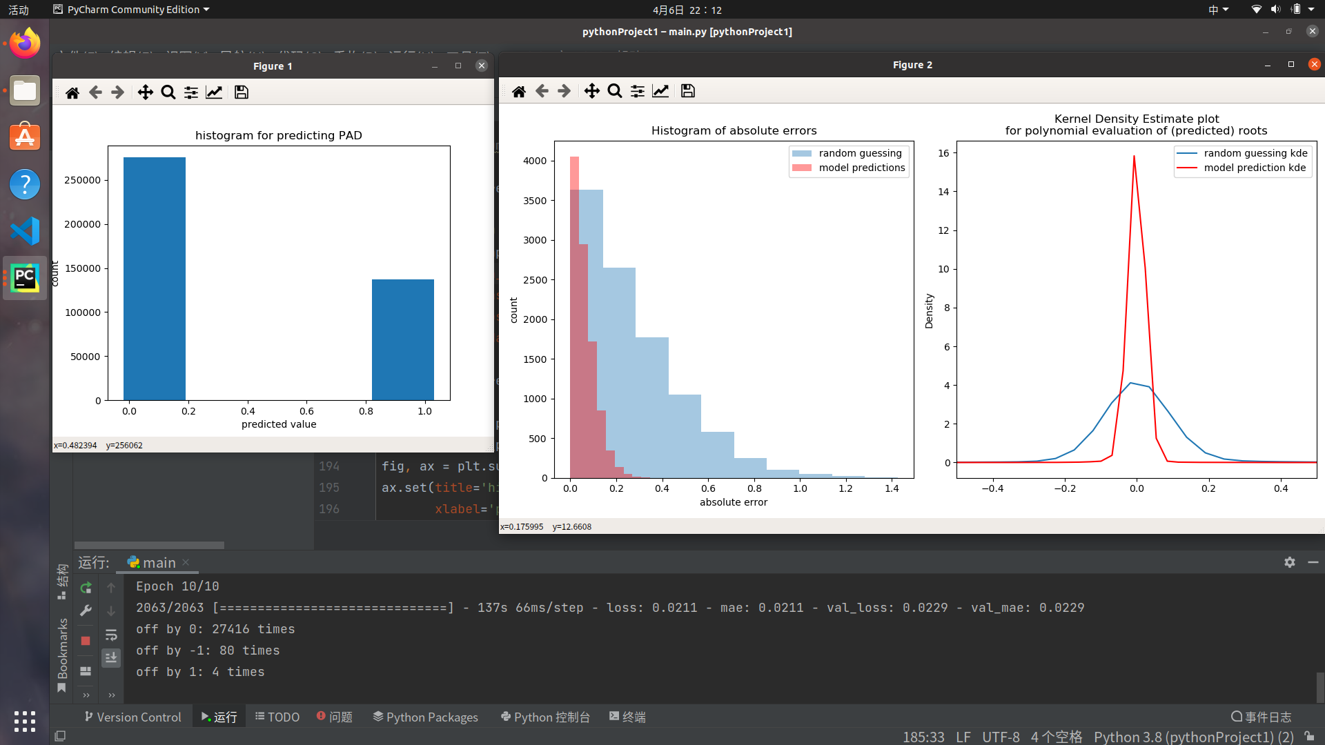
至此可以看出,经过较高数量的训练,
[En]
At this point, it can be seen that after a higher number of training,
核密度图显示明显的变化。
[En]
The nuclear density map showed obvious changes.
保留通过十次训练得到的模型,并控制变量调整测试数据。
[En]
Keep the model obtained by ten times of training, and control variables to adjust the test data.
调参
(reshape(X[100:150])

(reshape(X[100:110])

(reshape(X[100:102])

import torch

device = torch.device("cuda:0" if torch.cuda.is_available() else "cpu")

#inputs,target = inputs.to(device),target.to(device)

import numpy as np
import pandas as pd
import matplotlib.pyplot as plt
MIN_ROOT = -1
MAX_ROOT = 1

def make(n_samples, n_degree):
    global MIN_ROOT, MAX_ROOT
    y = np.random.uniform(MIN_ROOT, MAX_ROOT, (n_samples, n_degree))
    y.sort(axis=1)
    X = np.array([np.poly(_) for _ in y])
    return X, y

toy case
X, y = make(1, 2)

N_SAMPLES = 100000
DEGREE = 5
X_train, y_train = make(int(N_SAMPLES*0.8), DEGREE)
X_test, y_test = make(int(N_SAMPLES*0.2), DEGREE)

import os
os.environ['TF_CPP_MIN_LOG_LEVEL']='2'

def reshape(array):
    return np.expand_dims(array, -1)

from keras.models import Sequential
from keras.layers import LSTM, RepeatVector, Dense, TimeDistributed

hidden_size = 128

model = Sequential()

ENCODER PART OF SEQ2SEQ
model.add(LSTM(hidden_size, input_shape=(DEGREE+1, 1)))

DECODER PART OF SEQ2SEQ
model.add(RepeatVector(DEGREE))  # this determines the length of the output sequence
model.add((LSTM(hidden_size, return_sequences=True)))
model.add(TimeDistributed(Dense(1)))

model.compile(loss='mean_absolute_error',
              optimizer='adam',
              metrics=['mae'])
#model.to(device)
#print(model.summary())
'''
BATCH_SIZE = 128
model.fit(reshape(X_train),
          reshape(y_train),
          batch_size=BATCH_SIZE,
          epochs=3,
          verbose=1,
          validation_data=(reshape(X_test),
                           reshape(y_test)))

y_pred = model.predict(reshape(X_test))
y_pred = np.squeeze(y_pred)

#% matplotlib inline

def get_evals(polynomials, roots):
    evals = [
        [np.polyval(poly, r) for r in root_row]
        for (root_row, poly) in zip(roots, polynomials)
    ]
    evals = np.array(evals).ravel()
    return evals

def compare_to_random(y_pred, y_test, polynomials):
    y_random = np.random.uniform(MIN_ROOT, MAX_ROOT, y_test.shape)
    y_random.sort(axis=1)

    fig, axes = plt.subplots(1, 2, figsize=(12, 6))
    ax = axes[0]
    ax.hist(np.abs((y_random - y_test).ravel()),
            alpha=.4, label='random guessing')
    ax.hist(np.abs((y_pred - y_test).ravel()),
            color='r', alpha=.4, label='model predictions')
    ax.set(title='Histogram of absolute errors',
           ylabel='count', xlabel='absolute error')
    ax.legend(loc='best')

    ax = axes[1]
    random_evals = get_evals(polynomials, y_random)
    predicted_evals = get_evals(polynomials, y_pred)
    pd.Series(random_evals).plot.kde(ax=ax, label='random guessing kde')
    pd.Series(predicted_evals).plot.kde(ax=ax, color='r', label='model prediction kde')
    title = 'Kernel Density Estimate plot\n' \
            'for polynomial evaluation of (predicted) roots'
    ax.set(xlim=[-.5, .5], title=title)
    ax.legend(loc='best')

    fig.tight_layout()

compare_to_random(y_pred, y_test, X_test)
plt.show()

'''

MAX_DEGREE = 15
MIN_DEGREE = 5
MAX_ROOT = 1
MIN_ROOT = -1
N_SAMPLES = 10000 * (MAX_DEGREE - MIN_DEGREE + 1)

def make(n_samples, max_degree, min_degree, min_root, max_root):
    samples_per_degree = n_samples
    n_samples = samples_per_degree * (max_degree - min_degree + 1)
    X = np.zeros((n_samples, max_degree + 1))
    # XXX: filling the truth labels with ZERO??? EOS character would be nice
    y = np.zeros((n_samples, max_degree, 2))
    for i, degree in enumerate(range(min_degree, max_degree + 1)):
        y_tmp = np.random.uniform(min_root, max_root, (samples_per_degree, degree))
        y_tmp.sort(axis=1)
        X_tmp = np.array([np.poly(_) for _ in y_tmp])

        root_slice_y = np.s_[
                       i * samples_per_degree:(i + 1) * samples_per_degree,
                       :degree,
                       0]
        pad_slice_y = np.s_[
                      i * samples_per_degree:(i + 1) * samples_per_degree,
                      degree:,
                      1]
        this_slice_X = np.s_[
                       i * samples_per_degree:(i + 1) * samples_per_degree,
                       -degree - 1:]

        y[root_slice_y] = y_tmp
        y[pad_slice_y] = 1
        X[this_slice_X] = X_tmp
    return X, y

def make_this():
    global MAX_DEGREE, MIN_DEGREE, MAX_ROOT, MIN_ROOT, N_SAMPLES
    return make(N_SAMPLES, MAX_DEGREE, MIN_DEGREE, MIN_ROOT, MAX_ROOT)

from sklearn.model_selection import train_test_split

X, y = make_this()
X_train, X_test, y_train, y_test = train_test_split(X, y, test_size=0.25)
'''
print('X shapes', X.shape, X_train.shape, X_test.shape)
print('y shapes', y.shape, y_train.shape, y_test.shape)
print('-' * 80)
print('This is an example root sequence')
print(y[0])
'''
hidden_size = 128
model = Sequential()

model.add(LSTM(hidden_size, input_shape=(MAX_DEGREE+1, 1)))
model.add(RepeatVector(MAX_DEGREE))
model.add((LSTM(hidden_size, return_sequences=True)))
model.add(TimeDistributed(Dense(2)))

model.compile(loss='mean_absolute_error',
              optimizer='adam',
              metrics=['mae'])

#print(model.summary())

model.predict(reshape(X_test));  # this last semi-column will suppress the output.

'''
BATCH_SIZE = 40
model.fit(reshape(X_train), y_train,
          batch_size=BATCH_SIZE,
          epochs=10,
          verbose=1,
          validation_data=(reshape(X_test), y_test))
'''
model.predict(reshape(X[100:102]))

y_pred = model.predict(reshape(X_test))
pad_or_not = y_pred[:, :, 1].ravel()
fig, ax = plt.subplots()
ax.set(title='histogram for predicting PAD',
       xlabel='predicted value',
       ylabel='count')
ax.hist(pad_or_not, bins=5);

thr = 0.5

def how_many_roots(predicted):
    global thr
    return np.sum(predicted[:, 1] < thr)

true_root_count = np.array(list(map(how_many_roots, y_test)))
pred_root_count = np.array(list(map(how_many_roots, y_pred)))
from collections import Counter
for key, val in Counter(true_root_count - pred_root_count).items():
    print('off by {}: {} times'.format(key, val))

index = np.where(true_root_count == pred_root_count)[0]
index = np.random.choice(index, 1000, replace=False)

predicted_evals, random_evals = [], []
random_roots_list = []
predicted_roots_list = []
true_roots_list = []
for i in index:
    predicted_roots = [row[0] for row in y_pred[i] if row[1] < thr]
    true_roots = [row[0] for row in y_test[i] if row[1] == 0]
    random_roots = np.random.uniform(MIN_ROOT, MAX_ROOT, len(predicted_roots))
    random_roots = sorted(random_roots)
    random_roots_list.extend(random_roots)
    predicted_roots_list.extend(predicted_roots)
    true_roots_list.extend(true_roots)
    for predicted_root, random_root in zip(predicted_roots, random_roots):
        predicted_evals.append(
            np.polyval(X_test[i], predicted_root))
        random_evals.append(
            np.polyval(X_test[i], random_root))

assert len(true_roots_list) == len(predicted_roots_list)
assert len(random_roots_list) == len(predicted_roots_list)
true_roots_list = np.array(true_roots_list)
random_roots_list = np.array(random_roots_list)
predicted_roots_list = np.array(predicted_roots_list)
fig, axes = plt.subplots(1, 2, figsize=(12, 6))
ax = axes[0]
ax.hist(np.abs(random_roots_list - true_roots_list),
        alpha=.4, label='random guessing')
ax.hist(np.abs(predicted_roots_list - true_roots_list),
        color='r', alpha=.4, label='model predictions')
ax.set(title='Histogram of absolute errors',
       ylabel='count', xlabel='absolute error')
ax.legend(loc='best')

ax = axes[1]
pd.Series(random_evals).plot.kde(ax=ax, label='random guessing kde')
pd.Series(predicted_evals).plot.kde(ax=ax, color='r', label='model prediction kde')
title = 'Kernel Density Estimate plot\n' \
        'for polynomial evaluation of (predicted) roots'
ax.set(xlim=[-.5, .5], title=title)
ax.legend(loc='best')

fig.tight_layout()

plt.show()
ML3
CNN实战
google colab
Download the dataset
You may choose where to download the data.

Google Drive
!gdown --id '1awF7pZ9Dz7X1jn1_QAiKN-_v56veCEKy' --output food-11.zip

Dropbox
!wget https:

MEGA
!sudo apt install megatools
!megadl "https://mega.nz/#!zt1TTIhK!ZuMbg5ZjGWzWX1I6nEUbfjMZgCmAgeqJlwDkqdIryfg"

Unzip the dataset.

This may take some time.

!unzip -q food-11.zip

Import necessary packages.

import numpy as np
import torch
import torch.nn as nn
import torchvision.transforms as transforms
from PIL import Image
"ConcatDataset" and "Subset" are possibly useful when doing semi-supervised learning.

from torch.utils.data import ConcatDataset, DataLoader, Subset
from torchvision.datasets import DatasetFolder

This is for the progress bar.

from tqdm.auto import tqdm

It is important to do data augmentation in training.

However, not every augmentation is useful.

Please think about what kind of augmentation is helpful for food recognition.

train_tfm = transforms.Compose([
    # Resize the image into a fixed shape (height = width = 128)
    transforms.Resize((128, 128)),
    # You may add some transforms here.

    # ToTensor() should be the last one of the transforms.

    transforms.ToTensor(),
])

We don't need augmentations in testing and validation.

All we need here is to resize the PIL image and transform it into Tensor.

test_tfm = transforms.Compose([
    transforms.Resize((128, 128)),
    transforms.ToTensor(),
])

Batch size for training, validation, and testing.

A greater batch size usually gives a more stable gradient.

But the GPU memory is limited, so please adjust it carefully.

batch_size = 128

Construct datasets.

The argument "loader" tells how torchvision reads the data.

train_set = DatasetFolder("food-11/training/labeled", loader=lambda x: Image.open(x), extensions="jpg", transform=train_tfm)
valid_set = DatasetFolder("food-11/validation", loader=lambda x: Image.open(x), extensions="jpg", transform=test_tfm)
unlabeled_set = DatasetFolder("food-11/training/unlabeled", loader=lambda x: Image.open(x), extensions="jpg", transform=train_tfm)
test_set = DatasetFolder("food-11/testing", loader=lambda x: Image.open(x), extensions="jpg", transform=test_tfm)

Construct data loaders.

train_loader = DataLoader(train_set, batch_size=batch_size, shuffle=True, num_workers=8, pin_memory=True)
valid_loader = DataLoader(valid_set, batch_size=batch_size, shuffle=True, num_workers=8, pin_memory=True)
test_loader = DataLoader(test_set, batch_size=batch_size, shuffle=False)

class Classifier(nn.Module):
    def __init__(self):
        super(Classifier, self).__init__()
        # The arguments for commonly used modules:
        # torch.nn.Conv2d(in_channels, out_channels, kernel_size, stride, padding)
        # torch.nn.MaxPool2d(kernel_size, stride, padding)

        # input image size: [3, 128, 128]
        self.cnn_layers = nn.Sequential(
            nn.Conv2d(3, 64, 3, 1, 1),
            nn.BatchNorm2d(64),
            nn.ReLU(),
            nn.MaxPool2d(2, 2, 0),

            nn.Conv2d(64, 128, 3, 1, 1),
            nn.BatchNorm2d(128),
            nn.ReLU(),
            nn.MaxPool2d(2, 2, 0),

            nn.Conv2d(128, 256, 3, 1, 1),
            nn.BatchNorm2d(256),
            nn.ReLU(),
            nn.MaxPool2d(4, 4, 0),
        )
        self.fc_layers = nn.Sequential(
            nn.Linear(256 * 8 * 8, 256),
            nn.ReLU(),
            nn.Linear(256, 256),
            nn.ReLU(),
            nn.Linear(256, 11)
        )

def forward(self, x):
        # input (x): [batch_size, 3, 128, 128]
        # output: [batch_size, 11]

        # Extract features by convolutional layers.

        x = self.cnn_layers(x)

        # The extracted feature map must be flatten before going to fully-connected layers.

        x = x.flatten(1)

        # The features are transformed by fully-connected layers to obtain the final logits.

        x = self.fc_layers(x)
        return x

def get_pseudo_labels(dataset, model, threshold=0.65):
    # This functions generates pseudo-labels of a dataset using given model.

    # It returns an instance of DatasetFolder containing images whose prediction confidences exceed a given threshold.

    # You are NOT allowed to use any models trained on external data for pseudo-labeling.

    device = "cuda" if torch.cuda.is_available() else "cpu"

    # Construct a data loader.

    data_loader = DataLoader(dataset, batch_size=batch_size, shuffle=False)

    # Make sure the model is in eval mode.

    model.eval()
    # Define softmax function.

    softmax = nn.Softmax(dim=-1)

    # Iterate over the dataset by batches.

    for batch in tqdm(data_loader):
        img, _ = batch

        # Forward the data
        # Using torch.no_grad() accelerates the forward process.

        with torch.no_grad():
            logits = model(img.to(device))

        # Obtain the probability distributions by applying softmax on logits.

        probs = softmax(logits)

        # ---------- TODO ----------
        # Filter the data and construct a new dataset.

    # # Turn off the eval mode.

    model.train()
    return dataset

"cuda" only when GPUs are available.

device = "cuda" if torch.cuda.is_available() else "cpu"

Initialize a model, and put it on the device specified.

model = Classifier().to(device)
model.device = device

For the classification task, we use cross-entropy as the measurement of performance.

criterion = nn.CrossEntropyLoss()

Initialize optimizer, you may fine-tune some hyperparameters such as learning rate on your own.

optimizer = torch.optim.Adam(model.parameters(), lr=0.0003, weight_decay=1e-5)

The number of training epochs.

n_epochs = 80

Whether to do semi-supervised learning.

do_semi = False

for epoch in range(n_epochs):
    # ---------- TODO ----------
    # In each epoch, relabel the unlabeled dataset for semi-supervised learning.

    # Then you can combine the labeled dataset and pseudo-labeled dataset for the training.

    if do_semi:
        # Obtain pseudo-labels for unlabeled data using trained model.

        pseudo_set = get_pseudo_labels(unlabeled_set, model)

        # Construct a new dataset and a data loader for training.

        # This is used in semi-supervised learning only.

        concat_dataset = ConcatDataset([train_set, pseudo_set])
        train_loader = DataLoader(concat_dataset, batch_size=batch_size, shuffle=True, num_workers=8, pin_memory=True)

    # ---------- Training ----------
    # Make sure the model is in train mode before training.

    model.train()

    # These are used to record information in training.

    train_loss = []
    train_accs = []

    # Iterate the training set by batches.

    for batch in tqdm(train_loader):

        # A batch consists of image data and corresponding labels.

        imgs, labels = batch

        # Forward the data. (Make sure data and model are on the same device.)
        logits = model(imgs.to(device))

        # Calculate the cross-entropy loss.

        # We don't need to apply softmax before computing cross-entropy as it is done automatically.

        loss = criterion(logits, labels.to(device))

        # Gradients stored in the parameters in the previous step should be cleared out first.

        optimizer.zero_grad()

        # Compute the gradients for parameters.

        loss.backward()

        # Clip the gradient norms for stable training.

        grad_norm = nn.utils.clip_grad_norm_(model.parameters(), max_norm=10)

        # Update the parameters with computed gradients.

        optimizer.step()

        # Compute the accuracy for current batch.

        acc = (logits.argmax(dim=-1) == labels.to(device)).float().mean()

        # Record the loss and accuracy.

        train_loss.append(loss.item())
        train_accs.append(acc)

    # The average loss and accuracy of the training set is the average of the recorded values.

    train_loss = sum(train_loss) / len(train_loss)
    train_acc = sum(train_accs) / len(train_accs)

    # Print the information.

    print(f"[ Train | {epoch + 1:03d}/{n_epochs:03d} ] loss = {train_loss:.5f}, acc = {train_acc:.5f}")

    # ---------- Validation ----------
    # Make sure the model is in eval mode so that some modules like dropout are disabled and work normally.

    model.eval()

    # These are used to record information in validation.

    valid_loss = []
    valid_accs = []

    # Iterate the validation set by batches.

    for batch in tqdm(valid_loader):

        # A batch consists of image data and corresponding labels.

        imgs, labels = batch

        # We don't need gradient in validation.

        # Using torch.no_grad() accelerates the forward process.

        with torch.no_grad():
          logits = model(imgs.to(device))

        # We can still compute the loss (but not the gradient).

        loss = criterion(logits, labels.to(device))

        # Compute the accuracy for current batch.

        acc = (logits.argmax(dim=-1) == labels.to(device)).float().mean()

        # Record the loss and accuracy.

        valid_loss.append(loss.item())
        valid_accs.append(acc)

    # The average loss and accuracy for entire validation set is the average of the recorded values.

    valid_loss = sum(valid_loss) / len(valid_loss)
    valid_acc = sum(valid_accs) / len(valid_accs)

    # Print the information.

    print(f"[ Valid | {epoch + 1:03d}/{n_epochs:03d} ] loss = {valid_loss:.5f}, acc = {valid_acc:.5f}")
tensorflow基础
官方教程
https://www.tensorflow.org/guide/keras/sequential_model?hl=zh-cn
keras
设置
import tensorflow as tf
from tensorflow import keras
from tensorflow.keras import layers
Sequential
Sequential模型适用于层的普通堆栈,其中每层正好有一个输入张量和一个输出张量。
Define Sequential model with 3 layers
model = keras.Sequential(
    [
        layers.Dense(2, activation="relu", name="layer1"),
        layers.Dense(3, activation="relu", name="layer2"),
        layers.Dense(4, name="layer3"),
    ]
)
Call model on a test input
x = tf.ones((3, 3))
y = model(x)
顺序模型不适用于以下情况:
[En]
The sequential model is not appropriate in the following situations:
- 模型有多个输入或输出
[En]
the model has multiple inputs or outputs*
- 任何层都有多个输入或输出
[En]
any layer has multiple inputs or outputs*
- 您需要执行图层共享
- 您需要非线性拓扑(例如剩余连接、多分支模型)
[En]
you need nonlinear topologies (e.g. residual connections, multi-branch models)*
常见的调试工作流:add() + summary()
构建新的顺序体系结构时,以增量方式堆叠图层并频繁打印模型摘要非常有用。例如,这使您能够监视堆栈和图层如何缩减像素采样图像特征映射:add()Conv2DMaxPooling2D
model = keras.Sequential()
model.add(keras.Input(shape=(250, 250, 3)))  # 250x250 RGB images
model.add(layers.Conv2D(32, 5, strides=2, activation="relu"))
model.add(layers.Conv2D(32, 3, activation="relu"))
model.add(layers.MaxPooling2D(3))

Can you guess what the current output shape is at this point? Probably not.

Let's just print it:
model.summary()

The answer was: (40, 40, 32), so we can keep downsampling...

model.add(layers.Conv2D(32, 3, activation="relu"))
model.add(layers.Conv2D(32, 3, activation="relu"))
model.add(layers.MaxPooling2D(3))
model.add(layers.Conv2D(32, 3, activation="relu"))
model.add(layers.Conv2D(32, 3, activation="relu"))
model.add(layers.MaxPooling2D(2))

And now?

model.summary()

Now that we have 4x4 feature maps, time to apply global max pooling.

model.add(layers.GlobalMaxPooling2D())

Finally, we add a classification layer.

model.add(layers.Dense(10))
Eager Execution
TensorFlow 的 Eager Execution 是一种命令式编程环境,可立即评估运算,无需构建计算图:运算会返回具体的值,而非构建供稍后运行的计算图。这样能使您轻松入门 TensorFlow 并调试模型,同时也减少了样板代码。要跟随本指南进行学习,请在交互式 python 解释器中运行以下代码示例。
Eager Execution 是用于研究和实验的灵活机器学习平台,具备以下特性:
- 直观的界面 – 自然地组织代码结构并使用 Python 数据结构。快速迭代小模型和小数据。
- 更方便的调试功能 -直接调用运算以检查正在运行的模型并测试更改。使用标准 Python 调试工具立即报告错误。
- 自然的控制流 – 使用 Python而非计算图控制流,简化了动态模型的规范。
Eager Execution 支持大部分 TensorFlow 运算和 GPU 加速。
设置和基本用法
import os

import tensorflow as tf

import cProfile
Eager 训练
计算梯度
自动微分对实现机器学习算法(例如用于训练神经网络的反向传播)十分有用。在 Eager Execution 期间,请使用 tf.GradientTape 跟踪运算以便稍后计算梯度。
您可以在 Eager Execution 中使用 tf.GradientTape 来训练和/或计算梯度。这对复杂的训练循环特别有用。
由于在每次调用期间都可能进行不同运算,所有前向传递的运算都会记录到”条带”中。要计算梯度,请反向播放条带,然后丢弃。特定 tf.GradientTape 只能计算一个梯度;后续调用会引发运行时错误。
w = tf.Variable([[1.0]])
with tf.GradientTape() as tape:
  loss = w * w

grad = tape.gradient(loss, w)
print(grad)  # => tf.Tensor([[ 2.]], shape=(1, 1), dtype=float32)
训练模型
以下示例创建了一个多层模型,该模型会对标准 MNIST 手写数字进行分类。示例演示了在 Eager Execution 环境中构建可训练计算图的优化器和层 API。
Fetch and format the mnist data
(mnist_images, mnist_labels), _ = tf.keras.datasets.mnist.load_data()

dataset = tf.data.Dataset.from_tensor_slices(
  (tf.cast(mnist_images[...,tf.newaxis]/255, tf.float32),
   tf.cast(mnist_labels,tf.int64)))
dataset = dataset.shuffle(1000).batch(32)
Build the model
mnist_model = tf.keras.Sequential([
  tf.keras.layers.Conv2D(16,[3,3], activation='relu',
                         input_shape=(None, None, 1)),
  tf.keras.layers.Conv2D(16,[3,3], activation='relu'),
  tf.keras.layers.GlobalAveragePooling2D(),
  tf.keras.layers.Dense(10)
])
Original: https://blog.csdn.net/Algernon98/article/details/123993037
Author: 仿生程序员会梦见电子羊吗
Title: 【电子羊的奇妙冒险】初试深度学习(2)
原创文章受到原创版权保护。转载请注明出处:https://www.johngo689.com/508881/
转载文章受原作者版权保护。转载请注明原作者出处!