【PyTorch基础教程29】DIN模型

学习总结

• 推荐系统排序部分中的损失函数大部分都是二分类的交叉熵损失函数，但是召回的模型很多都不是。召回模型那块常见的还有sampled softmax损失函数；
• 模型训练时，在seed设置固定时模型的loss波动很大，可能是早停的次数太少了，也可能是​ ​batch_size​​比较小，导致数据不平衡，或者学习速率learning rate过大。

• DIN使用了一个local activation unit结构，利用候选商品和历史问题商品之间的相关性计算出权重，这个就代表了对于当前商品广告的预测，用户历史行为的各个商品的重要程度大小。

• 在rechub项目中，这个激活单元就是MLP，attention本质就是加权平均，MLP 是X@W，其中W是加权的权重，并且在MLP基础上多了softmax的条件（让权重之和为1）就是attention了。

• attention有很多种形式，比如transformer（点积形式）、DIN（MLP形式），只要最后得到一个注意力系数，就可以，通过反向传播机制，总会计算得到合适的权重。

文章目录

• ​​学习总结​​

• ​​一、数据特征表示​​

• ​​1.1 特征表示​​

• ​​二、深度兴趣网络DIN（add注意力）​​

• ​​2.1 用户行为特征 and 候选广告特征​​

• ​​2.2 累加每段用户行为序列​​

• ​​2.3 注意力机制的应用——DIN​​

• ​​（1）改进的地方​​

• ​​（2）激活单元（local activation unit）​​

• ​​三、代码部分​​

• ​​3.1 DIN模型部分​​

• ​​3.2 torch rechub的使用​​

• ​​（1）特征处理部分​​

• ​​（2）模型代码​​

• ​​四、几个问题​​

• ​​Reference​​

一、数据特征表示

1.1 特征表示

工业上的CTR预测数据集一般都是​ ​multi-group categorial form​​的形式，就是类别型特征最为常见，这种数据集一般长这样：

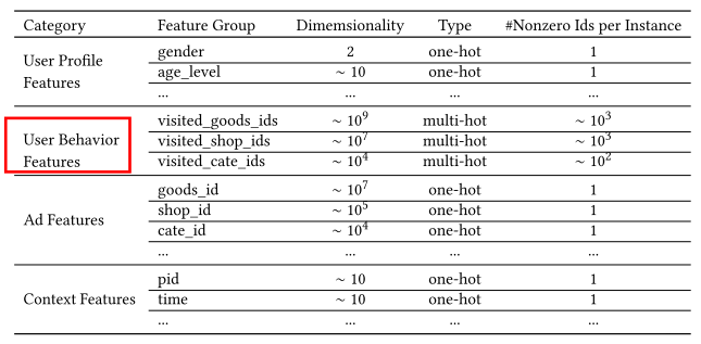
这里的亮点是边框功能，它包含了丰富的用户兴趣信息。

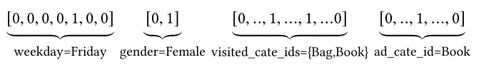
• 对于特征编码，作者这里举了个例子：​ ​[weekday=Friday, gender=Female, visited_cate_ids={Bag,Book}, ad_cate_id=Book]​​， 这种情况我们知道一般是通过one-hot的形式对其编码， 转成系数的二值特征的形式。
• 但是这里我们会发现一个​ ​visted_cate_ids​​， 也就是用户的历史商品列表， 对于某个用户来讲，这个值是个多值型的特征， 而且还要知道这个特征的长度不一样长，也就是用户购买的历史商品个数不一样多，这个显然。这个特征的话，我们一般是用到multi-hot编码，也就是可能不止1个1了，有哪个商品，对应位置就是1， 所以经过编码后的数据如下，送入模型：

上述功能没有互动组合，也就是没有功能交叉。这种交互信息被交给后来的神经网络学习。

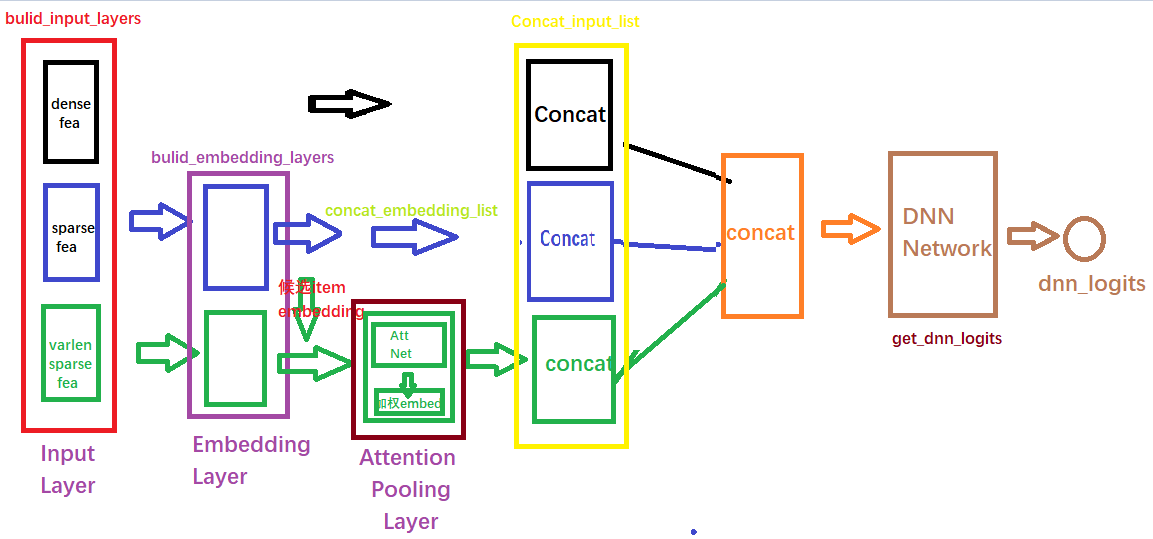
DIN模型的输入特征大致上分为了三类： Dense(连续型), Sparse(离散型), VarlenSparse(变长离散型)，也就是指的上面的历史行为数据。而不同的类型特征也就决定了后面处理的方式会不同：

• Dense型特征：由于是数值型了，这里为每个这样的特征建立Input层接收这种输入， 然后拼接起来先放着，等离散的那边处理好之后，和离散的拼接起来进DNN
• Sparse型特征，为离散型特征建立Input层接收输入，然后需要先通过embedding层转成低维稠密向量，然后拼接起来放着，等变长离散那边处理好之后， 一块拼起来进DNN， 但是这里面要注意有个特征的embedding向量还得拿出来用，就是候选商品的embedding向量，这个还得和后面的计算相关性，对历史行为序列加权。
• VarlenSparse型特征：这个一般指的用户的历史行为特征，变长数据， 首先会进行padding操作成等长， 然后建立Input层接收输入，然后通过embedding层得到各自历史行为的embedding向量， 拿着这些向量与上面的候选商品embedding向量进入AttentionPoolingLayer去对这些历史行为特征加权合并，最后得到输出。

在torch rechub项目中就是​ ​create_seq_features​​处理出对应的历史序列。

二、深度兴趣网络DIN（add注意力）

DIN 模型的应用场景是阿里最典型的电商广告推荐，有大量的用户历史行为信息（历史购买过得商品或类别信息）。对于付了广告费的商品，阿里会根据模型预测的点击率高低，把合适的广告商品推荐给合适的用户，所以 DIN 模型本质上是一个点击率预估模型。

下面的图 1 就是 DIN 的基础模型 Base Model。我们可以看到，Base Model 是一个典型的 Embedding MLP 的结构。它的输入特征有用户属性特征（User Proflie Features）、用户行为特征（User Behaviors）、候选广告特征（Candidate Ad）和场景特征（Context Features）。

图1 阿里Base模型的架构图 (出自论文 Deep Interest Network for Click-Through Rate Prediction)

2.1 用户行为特征 and 候选广告特征

前面已经提到了用户属性功能和场景功能。这里，请注意上图颜色部分的用户行为特征和候选广告特征：

（1）用户行为特征是由一系列用户购买过的商品组成的，也就是图上的 Goods 1 到 Goods N，而每个商品又包含了三个子特征，也就是图中的三个彩色点，其中红色代表商品 ID，蓝色是商铺 ID，粉色是商品类别 ID。
（2）候选广告特征也包含了这三个 ID 型的子特征，因为这里的候选广告也是一个阿里平台上的商品。

在深度学习中，一般只要遇到 ID 型特征，我们就构建它的 Embedding，然后把 Embedding 跟其他特征连接起来，输入后续的 MLP。

阿里的 Base Model 也是这么做的，它把三个 ID 转换成了对应的 Embedding，然后把这些 Embedding 连接起来组成了当前商品的 Embedding。

2.2 累加每段用户行为序列

因为用户的行为序列其实是一组商品的序列，这个序列可长可短，但是神经网络的输入向量的维度必须是固定的，那我们应该怎么把这一组商品的 Embedding 处理成一个长度固定的 Embedding 呢？如图 1 中的 SUM Pooling 层的结构，就是直接把这些商品的 Embedding 叠加起来（向量累加），然后再把叠加后的 Embedding 跟其他所有特征的连接结果输入 MLP。

【SUM Pooling的不足】
SUM Pooling 的 Embedding 叠加操作其实是把所有历史行为一视同仁，没有任何重点地加起来，这其实并不符合我们购物的习惯。

举个例子来说，候选广告对应的商品是”键盘”，与此同时，用户的历史行为序列中有这样几个商品 ID，分别是”鼠标””T 恤”和”洗面奶”。从我们的购物常识出发，”鼠标”这个历史商品 ID 对预测”键盘”广告点击率的重要程度应该远大于后两者。从注意力机制的角度出发，我们在购买键盘的时候，会把注意力更多地投向购买”鼠标”这类相关商品的历史上，因为这些购买经验更有利于我们做出更好的决策。

【基线模型各个模块】

• Embedding layer：把高维稀疏的输入转成低维稠密向量， 每个离散特征下面都会对应着一个embedding词典， 维度是， 这里的表示的是隐向量的维度， 而表示的是当前离散特征的唯一取值个数, 这里为了好理解，这里举个例子说明，就比如上面的weekday特征：

假设某个用户的weekday特征就是周五，化成one-hot编码的时候，就是[0,0,0,0,1,0,0]表示，这里如果再假设隐向量维度是D， 那么这个特征对应的embedding词典是一个的一个矩阵(每一列代表一个embedding，7列正好7个embedding向量，对应周一到周日)，那么该用户这个one-hot向量经过embedding层之后会得到一个的向量，也就是周五对应的那个embedding，怎么算的，其实就是
其实也就是直接把embedding矩阵中one-hot向量为1的那个位置的embedding向量拿出来。 这样就得到了稀疏特征的稠密向量了。其他离散特征也是同理，只不过上面那个multi-hot编码的那个，会得到一个embedding向量的列表，因为他开始的那个multi-hot向量不止有一个是1，这样乘以embedding矩阵，就会得到一个列表了。通过这个层，上面的输入特征都可以拿到相应的稠密embedding向量了。

• pooling layer and Concat layer：

• pooling层的作用是将用户的历史行为embedding这个最终变成一个定长的向量，因为每个用户历史购买的商品数是不一样的， 也就是每个用户multi-hot中1的个数不一致，这样经过embedding层，得到的用户历史行为embedding的个数不一样多，也就是上面的embedding列表不一样长， 那么这样的话，每个用户的历史行为特征拼起来就不一样长了。 而后面如果加全连接网络的话，我们知道，他需要定长的特征输入。 所以往往用一个pooling layer先把用户历史行为embedding变成固定长度(统一长度)，所以有了这个公式：

这里的是用户历史行为的那些embedding。就变成了定长的向量， 这里的表示第个历史特征组(是历史行为，比如历史的商品id，历史的商品类别id等)， 这里的表示对应历史特种组里面用户购买过的商品数量，也就是历史embedding的数量，看上面图里面的user behaviors系列，就是那个过程了。
* Concat layer层的作用就是拼接了，就是把这所有的特征embedding向量，如果再有连续特征的话也算上，从特征维度拼接整合，作为MLP的输入。

• MLP：普通的全连接，用了学习特征之间的各种交互。

CTR二分类任务中，一般损失函数用的负的log对数似然：

base模型的改进点：

• 综合来看，不再可能看到用户历史行为中的哪种产品与当前商品更相关，即历史行为中每种商品对当前预测的重要性损失。
  
  [En]

  taken together, it is no longer possible to see which product in the user’s historical behavior is more related to the current commodity, that is, the loss of the importance of each commodity in the historical behavior to the current forecast.*

• 最后一点就是如果所有用户浏览过的历史行为商品，最后都通过embedding和pooling转换成了固定长度的embedding，这样会限制模型学习用户的多样化兴趣。

具体的改进思路：

• 加大embedding的维度，增加之前各个商品的表达能力，这样即使综合起来，embedding的表达能力也会加强， 能够蕴涵用户的兴趣信息，但是这个在大规模的真实推荐场景计算量超级大，不可取。
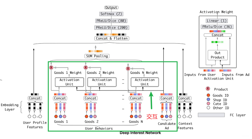
• 即DIN，在当前候选广告和用户的历史行为之间引入注意力的机制，这样在预测当前广告是否点击的时候，让模型更关注于与当前广告相关的那些用户历史产品，也就是说与当前商品更加相关的历史行为更能促进用户的点击行为。

2.3 注意力机制的应用——DIN

（1）改进的地方

所以阿里就在base model基础上，在用户的历史行为序列处理上应用注意力机制。

具体的操作如下图：DIN 为每个用户的历史购买商品加上了一个激活单元（Activation Unit）——这个激活单元生成了一个权重，这个权重就是用户对这个历史商品的注意力得分，权重的大小对应用户注意力的高低。

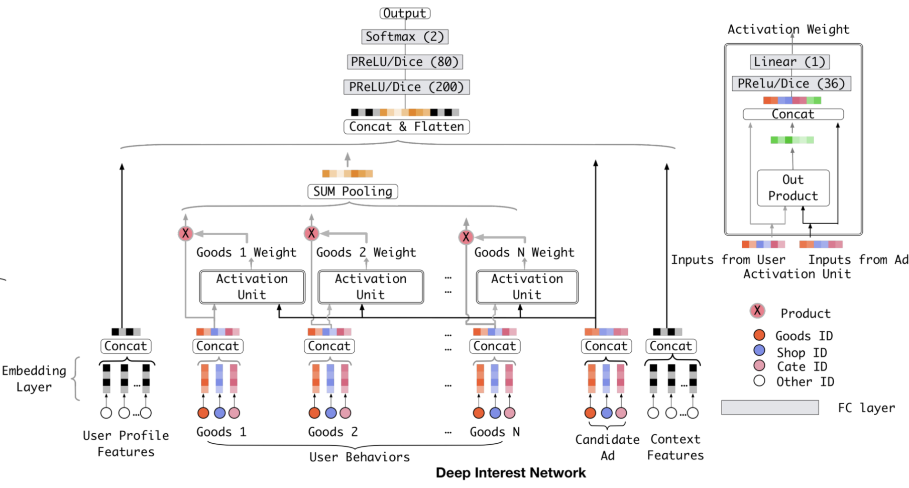
图3 阿里DIN模型的架构图 (出自论文 Deep Interest Network for Click-Through Rate Prediction)

再和之前的base模型对比：

图1 阿里Base模型的架构图 (出自论文 Deep Interest Network for Click-Through Rate Prediction)

（2）激活单元（local activation unit）

可以看到上面图3的右方的激活单元的详细结构：
input：当前这个历史行为商品的 Embedding，以及候选广告商品的 Embedding。
做法：把这两个输入 Embedding，与它们的外积结果连接起来形成一个向量（ 该向量方向是这个两个向量组成的平面的法向量方向），再输入给激活单元的 MLP 层，最终会生成一个注意力权重。

（1）激活单元就相当于一个小的深度学习模型，它利用两个商品的 Embedding，生成了代表它们关联程度的注意力权重。
（2）Sparrow里面的代码。没有严格意义上使用外积。使用的是​​ ​element-wise sub​​​ & ​ ​multipy​​​。然后用这两个向量去拼接，组成的​ ​activation_all​​​。
王喆的实践经验：外部产品的作用不是很大，大大增加了参数的数量。

[En]

Wang Zhe’s practical experience: the role of external product is not very great, and greatly increase the number of parameters.

local activation unit能根据用户历史行为特征和当前广告的相关性给用户历史行为特征embedding进行加权：里面是前馈神经网络，输入是用户历史行为商品和当前的候选商品， 输出是它俩之间的相关性， 这个相关性相当于每个历史商品的权重，把这个权重与原来的历史行为embedding相乘求和就得到了用户的兴趣表示，其公式：

以上公式的具体象征性解释：

• 是用户
• 表示的是候选广告
• 重量或历史行为商品和当前广告
  
  [En]

  weight or historical behavior goods and current advertisements*

• 除了历史行为向量和候选广告向量外，投入还有两者的外在产品运营。笔者认为，这是有助于模型相关性建模的显性知识。
  
  [En]

  in addition to the historical behavior vector and candidate advertising vector, the input also has an outer product operation of the two. The author says that this is explicit knowledge that is conducive to model correlation modeling.*

RecHub中的ActivationUnit代码：

class ActivationUnit(torch.nn.Module):    def __init__(self, emb_dim, dims=[36], activation="dice", use_softmax=False):        super(ActivationUnit, self).__init__()        self.emb_dim = emb_dim        self.use_softmax = use_softmax        # Dice(36)        self.attention = MLP(4 * self.emb_dim, dims=dims, activation=activation)    def forward(self, history, target):        seq_length = history.size(1)        target = target.unsqueeze(1).expand(-1, seq_length, -1)        # Concat        att_input = torch.cat([target, history, target - history, target * history], dim=-1)          # Dice(36)        att_weight = self.attention(att_input.view(-1, 4 * self.emb_dim))          # Linear(1)        att_weight = att_weight.view(-1, seq_length)        if self.use_softmax:            att_weight = att_weight.softmax(dim=-1)        # (batch_size,emb_dim)        output = (att_weight.unsqueeze(-1) * history).sum(dim=1)        return

其中可以看到在​ ​self.attention​​​赋值这里是用​ ​MLP​​：

class MLP(nn.Module):    """Multi Layer Perceptron Module, it is the most widely used module for     learning feature. Note we default add BatchNorm1d and Activation     Dropout for each Linear Module.    Args:        input dim (int): input size of the first Linear Layer.        output_layer (bool): whether this MLP module is the output layer. If True, then append one Linear(*,1) module.         dims (list): output size of Linear Layer (default=[]).        dropout (float): probability of an element to be zeroed (default = 0.5).        activation (str): the activation function, support [sigmoid, relu, prelu, dice, softmax] (default='relu').    Shape:        - Input: (batch_size, input_dim)        - Output: (batch_size, 1) or (batch_size, dims[-1])    """    def __init__(self, input_dim, output_layer=True, dims=[], dropout=0, activation="relu"):        super().__init__()        layers = list()        for i_dim in dims:            layers.append(nn.Linear(input_dim, i_dim))            layers.append(nn.BatchNorm1d(i_dim))            layers.append(activation_layer(activation))            layers.append(nn.Dropout(p=dropout))            input_dim = i_dim        if output_layer:            layers.append(nn.Linear(input_dim, 1))        self.mlp = nn.Sequential(*layers)    def forward(self, x):        return self.mlp(x)

三、代码部分

3.1 DIN模型部分

import torchimport torch.nn as nnimport numpy as npfrom torch.nn.modules.activation import Sigmoidclass DIN(nn.Module):    def __init__(self, candidate_movie_num, recent_rate_num, user_profile_num, context_feature_num, candidate_movie_dict,             recent_rate_dict, user_profile_dict, context_feature_dict, history_num, embed_dim, activation_dim, hidden_dim=[128, 64]):        super().__init__()        self.candidate_vocab_list = list(candidate_movie_dict.values())        self.recent_rate_list = list(recent_rate_dict.values())        self.user_profile_list = list(user_profile_dict.values())        self.context_feature_list = list(context_feature_dict.values())        self.embed_dim = embed_dim        self.history_num = history_num        # candidate_embedding_layer         self.candidate_embedding_list = nn.ModuleList([nn.Embedding(vocab_size, embed_dim) for vocab_size in self.candidate_vocab_list])        # recent_rate_embedding_layer        self.recent_rate_embedding_list = nn.ModuleList([nn.Embedding(vocab_size, embed_dim) for vocab_size in self.recent_rate_list])        # user_profile_embedding_layer        self.user_profile_embedding_list = nn.ModuleList([nn.Embedding(vocab_size, embed_dim) for vocab_size in self.user_profile_list])        # context_embedding_list        self.context_embedding_list = nn.ModuleList([nn.Embedding(vocab_size, embed_dim) for vocab_size in self.context_feature_list])        # activation_unit        self.activation_unit = nn.Sequential(nn.Linear(4*embed_dim, activation_dim),                                             nn.PReLU(),                                            nn.Linear(activation_dim, 1),                                            nn.Sigmoid())                # self.dnn_part        self.dnn_input_dim = len(self.candidate_embedding_list) * embed_dim + candidate_movie_num - len(            self.candidate_embedding_list) + embed_dim + len(self.user_profile_embedding_list) * embed_dim + \            user_profile_num - len(self.user_profile_embedding_list) + len(self.context_embedding_list) * embed_dim \            + context_feature_num - len(self.context_embedding_list)        self.dnn = nn.Sequential(nn.Linear(self.dnn_input_dim, hidden_dim[0]),                             nn.BatchNorm1d(hidden_dim[0]),                             nn.PReLU(),                             nn.Linear(hidden_dim[0], hidden_dim[1]),                             nn.BatchNorm1d(hidden_dim[1]),                             nn.PReLU(),                             nn.Linear(hidden_dim[1], 1),                             nn.Sigmoid())    def forward(self, candidate_features, recent_features, user_features, context_features):        bs = candidate_features.shape[0]        # candidate cate_feat embed        candidate_embed_features = []        for i, embed_layer in enumerate(self.candidate_embedding_list):            candidate_embed_features.append(embed_layer(candidate_features[:, i].long()))        candidate_embed_features = torch.stack(candidate_embed_features, dim=1).reshape(bs, -1).unsqueeze(1)        ## add candidate continous feat        candidate_continous_features = candidate_features[:, len(candidate_features):]        candidate_branch_features = torch.cat([candidate_continous_features.unsqueeze(1), candidate_embed_features], dim=2).repeat(1, self.history_num, 1)        # recent_rate  cate_feat embed        recent_embed_features = []        for i, embed_layer in enumerate(self.recent_rate_embedding_list):            recent_embed_features.append(embed_layer(recent_features[:, i].long()))        recent_branch_features = torch.stack(recent_embed_features, dim=1)                # user_profile feat embed         user_profile_embed_features = []        for i, embed_layer in enumerate(self.user_profile_embedding_list):            user_profile_embed_features.append(embed_layer(user_features[:, i].long()))        user_profile_embed_features = torch.cat(user_profile_embed_features, dim=1)        ## add user_profile continous feat        user_profile_continous_features = user_features[:, len(self.user_profile_list):]        user_profile_branch_features = torch.cat([user_profile_embed_features, user_profile_continous_features], dim=1)        # context embed feat        context_embed_features = []        for i, embed_layer in enumerate(self.context_embedding_list):            context_embed_features.append(embed_layer(context_features[:, i].long()))        context_embed_features = torch.cat(context_embed_features, dim=1)        ## add context continous feat        context_continous_features = context_features[:, len(self.context_embedding_list):]        context_branch_features = torch.cat([context_embed_features, context_continous_features], dim=1)        # activation_unit        sub_unit_input = recent_branch_features - candidate_branch_features        product_unit_input = torch.mul(recent_branch_features, candidate_branch_features)        unit_input = torch.cat([recent_branch_features, candidate_branch_features, sub_unit_input, product_unit_input], dim=2)        # weight-pool        activation_unit_out = self.activation_unit(unit_input).repeat(1, 1, self.embed_dim)        recent_branch_pooled_features = torch.mean(torch.mul(activation_unit_out, recent_branch_features), dim=1)        # dnn part        dnn_input = torch.cat([candidate_branch_features[:, 0, :], recent_branch_pooled_features, user_profile_branch_features, context_branch_features], dim=1)        dnn_out = self.dnn(dnn_input)        return

3.2 torch rechub的使用

比如在数据集​ ​amazon_electronics_sample​​上跑DIN模型。原数据是json格式，我们提取所需要的信息预处理为一个仅包含user_id, item_id, cate_id, time四个特征列的CSV文件：

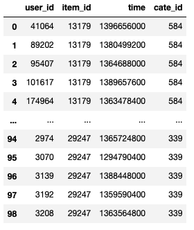
（1）特征处理部分

from torch_rechub.basic.features import DenseFeature, SparseFeature, SequenceFeaturen_users, n_items, n_cates = data["user_id"].max(), data["item_id"].max(), data["cate_id"].max()# 这里指定每一列特征的处理方式，对于sparsefeature，需要输入embedding层，所以需要指定特征空间大小和输出的维度features = [SparseFeature("target_item", vocab_size=n_items + 2, embed_dim=8),            SparseFeature("target_cate", vocab_size=n_cates + 2, embed_dim=8),            SparseFeature("user_id", vocab_size=n_users + 2, embed_dim=8)]target_features = features# 对于序列特征，除了需要和类别特征一样处理意外，item序列和候选item应该属于同一个空间，我们希望模型共享它们的embedding，所以可以通过shared_with参数指定history_features = [    SequenceFeature("history_item", vocab_size=n_items + 2, embed_dim=8, pooling="concat", shared_with="target_item"),    SequenceFeature("history_cate", vocab_size=n_cates + 2, embed_dim=8, pooling="concat", shared_with="target_cate")]

（2）模型代码

• 在基础数据集上要进行处理得到行为特征​ ​hist_behavior​​；
• 这种历史行为数据是序列特征，不同用户的历史行为特征长度不同，所以进入NN前我们一般会按照最长的序列进行padding；具体层上进行运算的时候，会用mask掩码的方式标记出这些填充的位置，好保证计算的准确性。

class DIN(torch.nn.Module):    def __init__(self, features, history_features, target_features, mlp_params, attention_mlp_params):        super().__init__()        self.features = features        self.history_features = history_features        self.target_features = target_features        # 历史行为特征个数        self.num_history_features = len(history_features)        # 计算所有的dim        self.all_dims = sum([fea.embed_dim for fea in features + history_features + target_features])                # 构建Embeding层        self.embedding = EmbeddingLayer(features + history_features + target_features)        # 构建注意力层        self.attention_layers = nn.ModuleList(            [ActivationUnit(fea.embed_dim, **attention_mlp_params) for fea in self.history_features])        self.mlp = MLP(self.all_dims, activation="dice", **mlp_params)    def forward(self, x):        embed_x_features = self.embedding(x, self.features)        embed_x_history = self.embedding(x, self.history_features)        embed_x_target = self.embedding(x, self.target_features)        attention_pooling = []        for i in range(self.num_history_features):            attention_seq = self.attention_layers[i](embed_x_history[:, i, :, :], embed_x_target[:, i, :])            attention_pooling.append(attention_seq.unsqueeze(1))         # SUM Pooling        attention_pooling = torch.cat(attention_pooling, dim=1)        # Concat & Flatten        mlp_in = torch.cat([            attention_pooling.flatten(start_dim=1),            embed_x_target.flatten(start_dim=1),            embed_x_features.flatten(start_dim=1)        ], dim=1)                # 可传入[80, 200]        y = self.mlp(mlp_in)                # 代码中使用的是sigmoid(1)+BCELoss，效果和论文中的DIN模型softmax(2)+CELoss类似        return torch.sigmoid(y.squeeze(1))

四、几个问题

• DIN模型在工业上的应用还是比较广泛的， 大家可以自由去通过查资料看一下具体实践当中这个模型是怎么用的？
• 例如，行为序列的产生是否合理，如果时间间隔长，是否应该进行分段？
  
  [En]

  for example, is the production of behavior sequence reasonable, and should it be divided into segments if the time interval is long?*

• 比如注意力机制那里能不能改成别的计算注意力的方式会好点？(我们也知道注意力机制的方式可不仅DNN这一种)， 再比如注意力权重那里该不该加softmax？

Reference

[1] ​​【CTR预估】CTR模型如何加入稠密连续型和序列型特征？​​​ [2] datawhale rechub项目
[3] 《深度学习推荐系统》王喆
[4] ​​DIN模型思维导图讲解​​

Original: https://blog.51cto.com/u_15717393/5471452
Author: wx62cea850b9e28
Title: 【PyTorch基础教程29】DIN模型