基于LSTM算法的股票预测

*
– 一、LSTM基本原理
–
+ 1.长短期记忆(LSTM)
– 二、LSTM预测股票走势
–
+ 1.导入相关库文件
+ 2.从oss2下载并解压数据集
+
* （1）关于oss的学习
* （2）具体代码及注释
+ 3.解压数据
+
* （1）关于解压命令
* （2）关于!rm -rf __MACOSX
* （3）具体代码及相关注释
+ 4.导入数据可视化
+
* （1）df.info():
* （2）head()函数的观察读取的数据
* （3）使用describe观察数据的分布情况
* （4）可视化选取的相关指标
+ 5.数据的预处理
+
* （1）数据集划分比例
* （2）定义最小最大值归一化函数
* （3）划分数据集
* （4）去除冗余指标并显示训练集的有效指标
* （5）归一化并查看训练集，验证集，测试集的大小
* （6）对指标数据可视化
+ 6.RNN建模-LSTM/GRU
+
* （1）对训练数据随机化处理
* （2）定义超参
* （3）定义网络结构
* （4）开始训练
+ 7.模型预测
+
* （1）模型的预测
* （2）预测结果可视化
+ 三、数据集与实验环境
+
* （1）数据集下载链接
* （2）环境配置
+ 四、总结
+ 1.混淆矩阵
+ 2.续前文LeNet5股票预测

一、LSTM基本原理

1.长短期记忆(LSTM)

LSTM是一种循环神经网络(RNN)，可学习时间步长序列和数据之间的长期依赖关系，与CNN不同，LSTM可以记住预测之间的网络状态。
LSTM适用于序列和时序数据分类，此时必须基于记忆的数据点序列进行网络预测或输出。股票是随着时间变化的，恰好可以用LSTM。

二、LSTM预测股票走势

1.导入相关库文件

import numpy as np
import pandas as pd
import math
import sklearn
import sklearn.preprocessing
import datetime
import os
import matplotlib.pyplot as plt
import tensorflow as tf

2.从oss2下载并解压数据集

（1）关于oss的学习

oss_getenv()用于获取环境变量的值（存在），否则返回默认值

获取环境变量，或设置类似“

（2）具体代码及注释

import oss2
access_key_id = os.getenv('OSS_TEST_ACCESS_KEY_ID','LTAI4G1MuHTUeNrKdQEPnbph')
access_key_secret = os.getenv('OSS_TEST_ACCESS_KEY_SECRET','m1ILSoVqcPUxFFDqer4tKDxDkoP1ji')
bucket_name = os.getenv('OSS_TEST_BUCKET','mldemo')
endpoint = os.getenv('OSS_TEST_ENDPOINT','https://oss-cn-shanghai.aliyuncs.com')

bucket = oss2.Bucket(oss2.Auth(access_key_id,access_key_secret),endpoint,bucket_name)

bucket.get_object_to_file('data/c12/stock_data.zip','stock_data.zip')

3.解压数据

（1）关于解压命令

unzip命令常用参数
-l：显示压缩文件内所包含的文件；
-t：检查压缩文件是否正确；
-o：不必先询问用户，unzip执行后覆盖原有的文件；
·-n：解压缩时不要覆盖原有的文件；

-q：执行时不显示任何信息；

-d

（2）关于!rm -rf __MACOSX

• rm -rf * 删除当前目录下的所有文件

压缩文件夹里边的 __MACOSX是缓存文件，可以直接删除掉

• __MACOSX的由来

Mac在压缩文件时会往里面写入MetaData，这样做的目的是为了方便其他的Mac用户使用，就想Windows会在图片目录中加入的Thumbs.db，以方便显示预览图一样

这些MetaData产生的文件就是 __MACOSX，本身这些文件在Mac上是隐藏属性的，也确实方便了Mac用户

但在Windows中 __MACOSX就成了”缓存文件”或垃圾文件，只有在Windows系统才能看到，Mac不可见

所以，当我们打开压缩文件的时候，如果出现 __MACOSX，直接删除即可，不会对你的文件有任何影响

（3）具体代码及相关注释

!unzip -o -q stock_data.zip

!rm -rf __MACOSX

!ls stock_data -ilht

4.导入数据可视化

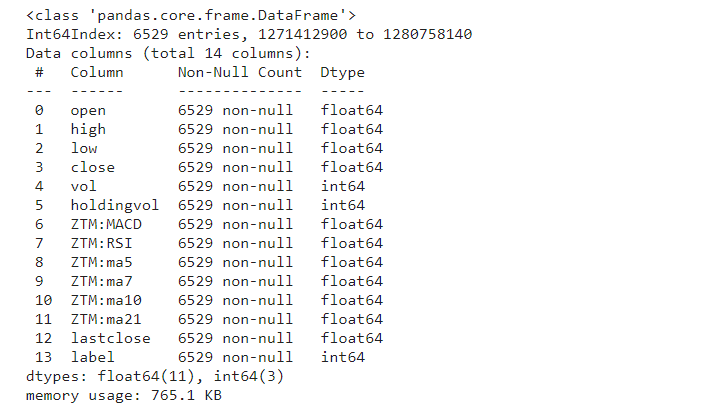
（1）df.info():

本文主要介绍了数据集的每一列的数据类型，是否为空，以及内存使用情况。

df = pd.read_csv("./stock_data/sh300index.csv",index_col = 0)

df.info()

运行结果

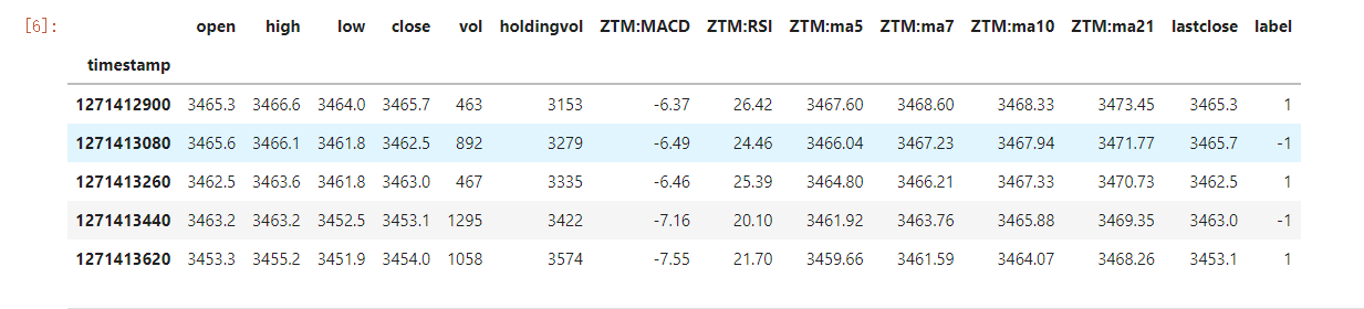
（2）head()函数的观察读取的数据

df.head()

运行结果：

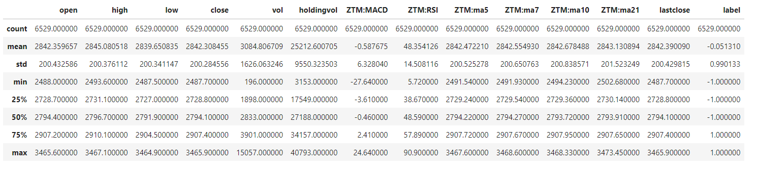
（3）使用describe观察数据的分布情况

df.describe()

运行结果：

（4）可视化选取的相关指标

plt.figure(figsize=(15,5));
plt.subplot(2,1,1);
plt.plot(df.open.values,color='red',label='open')
plt.plot(df.close.values,color='green',label='close')
plt.plot(df.low.values,color='blue',label='low')
plt.plot(df.high.values,color='black',label='high')
plt.title('stock price')
plt.xlabel('time [days]')
plt.ylabel('price')

plt.legend(loc = 'best')

plt.subplot(2,1,2)
plt.plot(df.vol.values,color='black',label='volume')
plt.title('stock volume')
plt.xlabel('time [days]')
plt.ylabel('volume')
plt.legend(loc = 'best')
plt.show()

运行结果：
上图显示了该股四个指标随时间的趋势图，下图显示了一段时间内股票交易量的趋势图。可以看出，当股价下跌时，股票交易量减少。

5.数据的预处理

（1）数据集划分比例

按照80%数据集，10%划分验证集，10%测试集对数据集进行划分。

valid_set_size_percentage = 10
test_set_size_percentage = 10

（2）定义最小最大值归一化函数

def normalize_data(df):
    min_max_scaler = sklearn.preprocessing.MinMaxScaler()
    df['open'] = min_max_scaler.fit_transform(df.open.values.reshape(-1,1))
    df['high'] = min_max_scaler.fit_transform(df.high.values.reshape(-1,1))
    df['low'] = min_max_scaler.fit_transform(df.low.values.reshape(-1,1))
    df['high'] = min_max_scaler.fit_transform(df['close'].values.reshape(-1,1))
    return df

（3）划分数据集

def load_data(stock,seq_len):
    data_raw = stock.to_numpy()
    data = []

    for index in range(len(data_raw)-seq_len):
        data.append(data_raw[index: index+seq_len])

    data = np.array(data);
    valid_set_size = int(np.round(valid_set_size_percentage/100*data.shape[0]));
    test_set_size = int(np.round(test_set_size_percentage/100*data.shape[0]));
    train_set_size = data.shape[0] - (valid_set_size + test_set_size);

    x_train = data[:train_set_size,:-1,:]
    y_train = data[:train_set_size,-1,:]

    x_valid = data[train_set_size:train_set_size+valid_set_size,:-1,:]
    y_valid = data[train_set_size:train_set_size+valid_set_size,-1,:]

    x_test = data[train_set_size+valid_set_size:,:-1,:]
    y_test = data[train_set_size+valid_set_size:,-1,:]

    return [x_train,y_train,x_valid,y_valid,x_test,y_test]

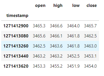
（4）去除冗余指标并显示训练集的有效指标

df_stock = df.copy()
df_stock.drop(['vol'],1,inplace=True)
df_stock.drop(['lastclose'],1,inplace=True)
df_stock.drop(['label'],1,inplace=True)
df_stock.drop(['ZTM:ma5'],1,inplace=True)
df_stock.drop(['ZTM:ma7'],1,inplace=True)
df_stock.drop(['ZTM:ma10'],1,inplace=True)
df_stock.drop(['ZTM:ma21'],1,inplace=True)
df_stock.drop(['holdingvol'],1,inplace=True)
df_stock.drop(['ZTM:MACD'],1,inplace=True)
df_stock.drop(['ZTM:RSI'],1,inplace=True)

df_stock.head()

运行结果：

（5）归一化并查看训练集，验证集，测试集的大小

df_stock_norm = normalize_data(df_stock)

seq_len = 20
x_train, y_train, x_valid,y_valid,x_test,y_test = load_data(df_stock_norm,seq_len)
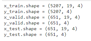
print('x_train.shape =',x_train.shape)
print('y_train.shape =',y_train.shape)
print('x_valid.shape =',x_valid.shape)
print('y_valid.shape =',y_valid.shape)
print('x_test.shape =',x_test.shape)
print('y_test.shape =',y_test.shape)

运行结果：

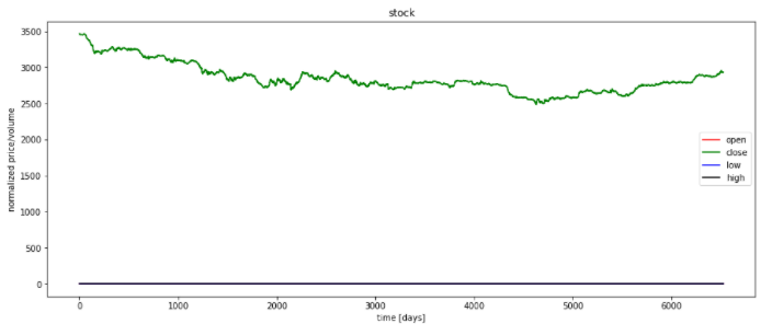
（6）对指标数据可视化

plt.figure(figsize=(15, 6));
plt.plot(df_stock_norm.open.values,color='red',label='open')
plt.plot(df_stock_norm.close.values,color='green',label='close')
plt.plot(df_stock_norm.low.values,color='blue',label='low')
plt.plot(df_stock_norm.high.values,color='black',label='high')
plt.title('stock')
plt.xlabel('time [days]')
plt.ylabel('normalized price/volume')
plt.legend(loc='best')
plt.show()

运行结果：

6.RNN建模-LSTM/GRU

（1）对训练数据随机化处理

index_in_epoch = 0;
perm_array = np.arange(x_train.shape[0])
np.random.shuffle(perm_array)

def get_next_batch(batch_size):
    global index_in_epoch,x_train,perm_array
    start = index_in_epoch
    index_in_epoch += batch_size

    if index_in_epoch > x_train.shape[0]:
        np.random.shuffle(perm_array)
        start = 0
        index_in_epoch = batch_size

    end = index_in_epoch
    return x_train[perm_array[start:end]],y_train[perm_array[start:end]]

（2）定义超参

n_steps = seq_len-1

n_inputs = 4
n_neurons =200

n_outputs = 4

n_layers = 2

learning_rate =0.001

batch_size = 50

n_epochs = 20

train_set_size = x_train.shape[0]

test_set_size = x_test.shape[0]

（3）定义网络结构

tf.reset_default_graph()

X = tf.placeholder(tf.float32, [None, n_steps, n_inputs])
y = tf.placeholder(tf.float32, [None, n_outputs])

layers = [tf.contrib.rnn.GRUCell(num_units=n_neurons, activation=tf.nn.leaky_relu)
         for layer in range(n_layers)]

multi_layer_cell = tf.contrib.rnn.MultiRNNCell(layers)
rnn_outputs, states = tf.nn.dynamic_rnn(multi_layer_cell, X, dtype=tf.float32)

stacked_rnn_outputs = tf.reshape(rnn_outputs, [-1, n_neurons])
stacked_outputs = tf.layers.dense(stacked_rnn_outputs, n_outputs)
outputs = tf.reshape(stacked_outputs, [-1, n_steps, n_outputs])
outputs = outputs[:,n_steps-1,:]

loss = tf.reduce_mean(tf.square(outputs - y))
optimizer = tf.train.AdamOptimizer(learning_rate=learning_rate)
training_op = optimizer.minimize(loss)

（4）开始训练

with tf.Session() as sess:
    sess.run(tf.global_variables_initializer())
    for iteration in range(int(n_epochs*train_set_size/batch_size)):
        x_batch, y_batch = get_next_batch(batch_size)
        sess.run(training_op, feed_dict={X: x_batch, y: y_batch})
        if iteration % int(5*train_set_size/batch_size) == 0:
            mse_train = loss.eval(feed_dict={X: x_train, y: y_train})
            mse_valid = loss.eval(feed_dict={X: x_valid, y: y_valid})
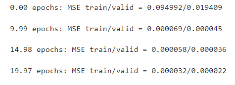
            print('%.2f epochs: MSE train/valid = %.6f/%.6f'%(
                iteration*batch_size/train_set_size, mse_train, mse_valid))

    y_train_pred = sess.run(outputs, feed_dict={X: x_train})
    y_valid_pred = sess.run(outputs, feed_dict={X: x_valid})
    y_test_pred = sess.run(outputs, feed_dict={X: x_test})

运行结果：
可以看出，训练集的均方误差损失已经减少到0.000032，验证集的均方误差已经减少到0.000022。

7.模型预测

（1）模型的预测

ft = 0

plt.figure(figsize=(15, 5));
plt.subplot(1,2,1);

plt.plot(np.arange(y_train.shape[0]), y_train[:,ft], color='blue', label='train target')

plt.plot(np.arange(y_train.shape[0], y_train.shape[0]+y_valid.shape[0]), y_valid[:,ft],
         color='gray', label='valid target')

plt.plot(np.arange(y_train.shape[0]+y_valid.shape[0],
                   y_train.shape[0]+y_test.shape[0]+y_test.shape[0]),
         y_test[:,ft], color='black', label='test target')

plt.plot(np.arange(y_train_pred.shape[0]),y_train_pred[:,ft], color='red',
         label='train prediction')

plt.plot(np.arange(y_train_pred.shape[0], y_train_pred.shape[0]+y_valid_pred.shape[0]),
         y_valid_pred[:,ft], color='orange', label='valid prediction')

plt.plot(np.arange(y_train_pred.shape[0]+y_valid_pred.shape[0],
                   y_train_pred.shape[0]+y_valid_pred.shape[0]+y_test_pred.shape[0]),
         y_test_pred[:,ft], color='green', label='test prediction')

plt.title('past and future stock prices')
plt.xlabel('time [days]')
plt.ylabel('normalized price')
plt.legend(loc='best');

plt.subplot(1,2,2);

plt.plot(np.arange(y_train.shape[0], y_train.shape[0]+y_test.shape[0]),
         y_test[:,ft], color='black', label='test target')

plt.plot(np.arange(y_train_pred.shape[0], y_train_pred.shape[0]+y_test_pred.shape[0]),
         y_test_pred[:,ft], color='green', label='test prediction')

plt.title('future stock prices')
plt.xlabel('time [days]')
plt.ylabel('normalized price')
plt.legend(loc='best');

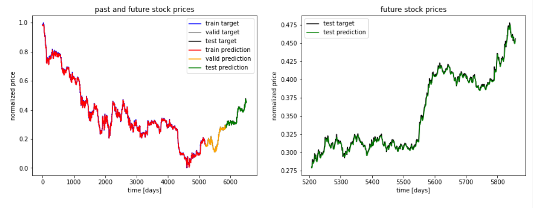
（2）预测结果可视化

左图：红色曲线为训练集的预测结果，橙色为验证集的预测结果，绿色为测试集的预测结果，右图显示了预测结果与测试集真实值的拟合关系。我们可以看到，拟合效果非常好。

; 三、数据集与实验环境

（1）数据集下载链接

https://download.csdn.net/download/fencecat/85104287

（2）环境配置

本实验使用tensorflow环境为1.14，如果安装的是tensorflow2.0版本会报错。

四、总结

1.混淆矩阵

• 事实上，我们可以使用混淆矩阵来可视化模型的训练精度。基本上，混淆矩阵显示有多少数据点实际属于一个类，而预测属于一个类。
  
  [En]

  in fact, we can use the confusion matrix to visualize the training accuracy of the model. Basically, the confusion matrix shows how many data points actually belong to one class, and the prediction belongs to one class.*

• 此外，还可以通过ROC曲线来判断模型是否有效。
• 通过混淆矩阵的可视化结果，我们可以比较基于深度学习算法LeNet5结构的股票预测与基于LSTM的股票预测的准确度，有兴趣的可以实现一下，这也是我下一步的任务。

2.续前文LeNet5股票预测

原文链接：https://blog.csdn.net/fencecat/article/details/124072324?spm=1001.2014.3001.5501
LeNet5股票预测文末的混淆矩阵实现模型精度可视化：

def plot_confusion_matrix(cm, labels_name, title):
    cm = cm.astype(np.float64)
    if(cm.sum(axis=0)[0]!=0):
        cm[:,0] = cm[:,0] / cm.sum(axis=0)[0]
    if(cm.sum(axis=0)[1]!=0):
        cm[:,1] = cm[:,1] / cm.sum(axis=0)[1]
    plt.imshow(cm, interpolation='nearest')
    plt.title(title)
    plt.colorbar()
    num_local = np.array(range(len(labels_name)))
    plt.xticks(num_local, labels_name)
    plt.yticks(num_local, labels_name)
    plt.ylabel('True label')
    plt.xlabel('Predicted label')
cm=confusion_matrix(t,pre)
y_true = np.array(list(map(int,t)))
y_scores = np.array(list(map(int,pre)))

roc=str(roc_auc_score(y_true, y_scores))
precision, recall, _thresholds = precision_recall_curve(y_true, y_scores)
pr =str(auc(recall, precision))
title="ROC AUC:"+roc+"\n"+"PR AUC:"+pr
labels_name=["0.0","1.0"]
plot_confusion_matrix(cm, labels_name, title)
for x in range(len(cm)):
    for y in range(len(cm[0])):
        plt.text(y,x,cm[x][y],color='white',fontsize=10, va='center')
plt.show()

可视化结果：

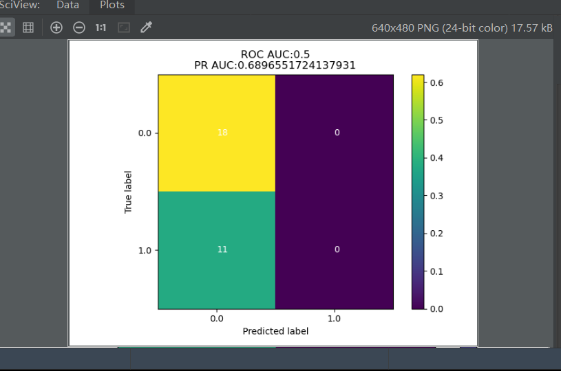
可以看到实验准确率为68.9%，并不是很好，可以通过调整网络结构优化模型来提高准确度。

Original: https://blog.csdn.net/fencecat/article/details/124081814
Author: Zkaisen
Title: 基于LSTM算法的股票预测